Example 4: Estimation Over a Network
In this example, a physical plant, its output digitally transmitted through a network, and a state estimator are modeled in Simulink as a hybrid system.
Contents
The files for this example are found in the package hybrid.examples.network_estimation :
- initialize.m
- network_est.slx
- postprocess.m
The contents of this package are located in Examples\+hybrid\+examples\network_estimation (clicking this link changes your working directory).
Mathematical Model
Consider a physical process given in terms of the state-space model
\[\begin{array}{l} \dot{x}=A x,\\ y= M x \end{array} \]
where \(x \in \mathbb{R}^{n_P}\) is the state and \(y \in \mathbb{R}^{r_P}\) is the measured output. The output is digitally transmitted through a network. At the other end of the network, a computer receives the information and runs an algorithm that takes the measurements of \(y\) to estimate the state \(x\) of the physical process.
We consider an estimation algorithm with a state variable \(\hat{x} \in \mathbb{R}^{n_P}\) , which denotes the estimate of \(x\) , that is appropriately reset to a new value involving the information received. More precisely, denoting the transmission times by \(t_i\) and \(L\) a constant matrix to be designed, the estimation algorithm updates its state as follows
\[\hat{x}^+=\hat{x}+L(y-M\hat{x}) \]
at every instant information is received. In between such events, the algorithm updates its state continuously so as to match the evolution of the state of the physical process, that is, via
\[\dot{\hat{x}} = A \hat{x} \]
Modeling the network as a hybrid system, which, in particular, assumes zero transmission delay, the state variables of the entire system are \(j_N\) , \(\tau_N \in \mathbb{R}\) , \(m_N \in \mathbb{R}^{r_P}\) , and \(x,\ \hat{x}\in \mathbb{R}^{n_P}\) . Then, transmissions occur when \(\tau_N \leq 0\) , at which events the state of the network is updated via
\[\tau_N^+ \in [T^{*\min}_{N},T^{*\max}_{N}],\quad j_N^+ = j_N+1, \qquad m_N^+ = y \]
and the state of the algorithm is updated via \(\hat{x}^+=\hat{x}+L(y-M\hat{x})\) . Note that since the state of the physical process does not change at such events, we can use the following trivial difference equation to update it at the network events:
\[x^+ = x \]
In between events, the state of the network is updated as
\[\dot{\tau}_N = -1, \qquad \dot{j}_N,\dot{m}_N = 0 \]
the state of the algorithm changes continuously according to \(\dot{\hat{x}} = A \hat{x}\) , and the state of the physical process changes according to \(\dot{x}=A x , y= M x\) . Based on the equations above, we pick the following data for each of the subsystems in the Simulink Model:
Physical process:
\[ \begin{array}{l@{}l} f_P(x, u):= Ax + Bu, \quad &C_P := \mathbb{R}^{n_p}\times\mathbb{R}, \\ G_P(x, u):= x, \quad &D_P := \emptyset,\\ y = h(x) := Mx \end{array}\]
where
\[\begin{array}{l@{}l} A=\left[\begin{array}{cccc} 0 & 1 & 0 & 0 \\ -1 & 0 & 0 & 0 \\ -2 & 1 & -1 & 0 \\ 2 & -2 & 0 & -2 \end{array}\right],\quad B = \left[\begin{array}{c} 0\\0\\1\\0 \end{array}\right],\quad M = \left[\begin{array}{cccc}1&0&0&0\end{array}\right], \end{array}\]
\(n_p=4\) , \(r_p=1\) , \(x \in\mathbb{R}^{n_p}\) , \(y\in\mathbb{R}^{r_p}\) , and \(u\in\mathbb{R}\) .
Network:
\[\begin{array}{l@{}l} f(x_N, u_N):= \left[\begin{array}{c} 0\\0\\-1 \end{array}\right],\quad &C := \{(x_N,u_N)\mid \tau_N \geq 0 \},\\ g(x_N, u_N):= \left[\begin{array}{c} u_N \\ j_N + 1 \\ \tau_r \end{array}\right],\quad &D :=\{(x_N,u_N)\mid \tau_N \leq 0 \},\\ y_N = h(x_N) : =x_N \end{array}\]
where
\(\tau_r\in[T^{*\min}_{N},T^{*\max}_{N}]\) is a random variable that models the time in-between communication instances. Also, the sate and the input are given by \(x_N=(m_N,j_N,\tau_N)\in\mathbb{R}\times\mathbb{R}\times\mathbb{R}\) , and \(u_N=y\in\mathbb{R}^{r_p}\) , respectively.
Estimator:
\[\begin{array}{ll} f(x_E, u_E):= \left[\begin{array}{cc} A & 0 \\ 0 & 0 \end{array}\right]x_E + \left[\begin{array}{c} B \\ 0 \end{array}\right]v,\quad & C := \{(x_E,u_E) \mid j_E = j_N \},\\ g((\hat{x},j_E), u_E):= \left[\begin{array}{c} \hat{x} + L(m_N-M\hat{x}) \\ j_N \end{array}\right],\quad &D :=\{(x,u) \mid j_E\in\mathbb{N}\setminus j_N\}, \end{array}\]
where \(L\) , which is designed as in [1], is given by
\[\begin{array}{l} L := \left[\begin{array}{c} 1 \\ -0.9433\\ -0.6773\\1.6274 \end{array}\right], \end{array}\]
the input and the state are given by \(u_E = (x_N,v) = ((m_N,j_N,\tau_N),v)\in\mathbb{R}\times\mathbb{R}\times\mathbb{R}\times\mathbb{R}\) , and \(x_E=(\hat{x},j_E)\in\mathbb{R}^{4}\times\mathbb{R}\) , respectively. Notice that the estimator block (Estimator) in the Simulink Model is implemented using a regular hybrid system block with embedded functions.
For each hybrid system in the Simulink Model (Continuous Process, network, and Estimator) we have the following Matlab embedded functions that describe the sets \(C\) and \(D\) and functions \(f\) and \(g\) .
Steps to Run Model
The following procedure is used to simulate the example using the model in the file network_est.slx :
- Open network_est.slx in Simulink.
- Double-click the block labeled Double Click to Initialize .
- To start the simulation, click the run button or select Simulation>Run .
- Once the simulation finishes, click the block labeled Double Click to Plot Solutions . Several plots of the computed solution will open.
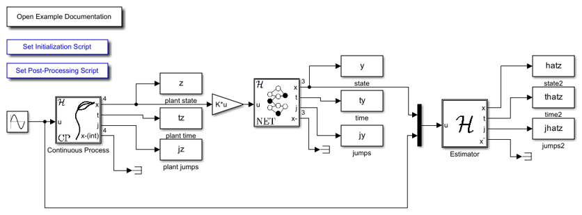
Simulink Model
The following diagram shows the Simulink model of the estimator over a network example. The contents of the blocks flow map f , flow set C , etc., are shown below. When the Simulink model is open, the blocks can be viewed and modified by double clicking on them.
The Simulink blocks for the hybrid systems in this example are included below.
Continuous Process:
flow map f block
function zdot = f(z, u, parameters)
    % Flow map for Estimation over a network

    A = parameters.A;
    B = parameters.B;

    zdot = A*z + B*u;
end
flow set C block
function inC = C(x, u, parameters) %#ok% Flow set indicator function. inC = 1; end
For more info about Continuous-time Plant blocks, such as Continuous Process , see here .
Network:
flow map f block
function xdot = f(x, u)
    % Network flow map
    n = length(u); % measured input size

    msdot = zeros(n,1); % measured continuous dynamics
    jdot = 0;
    tau_sdot = -1; % Timer tau_s
    xdot = [msdot; jdot; tau_sdot];
end
flow set C block
function inC = C(x, vs, T_max)
    % Flow set indicator function
    tau_s = x(end); % timer state

    if tau_s >= 0 && tau_s <= T_max
        inC = 1; % report flow
    elseif tau_s> T_max
        inC = 0; % do not report flow
    else
        inC = 0;
    end
end
jump map g block
function xplus = g(x, vs, measurement_times)
    % Jump map for network.

    n = length(vs); % input size
    j = x(n+1);
    msplus = vs; % output = measured input
    % The value tau_s is updated as a function of vs.
    tau_splus = measurement_times(j+1); % Timer tau_s
    j_plus = j+1;
    xplus = [msplus; j_plus; tau_splus];
end
jump set D block
function inD  = D(x, vs)
    % Jump set indicator function for network
    tau_s = x(end); % timer state

    if tau_s>=0
        inD = 0; % do not report jump
    elseif tau_s<= 0
        inD = 1; % report jump
    else
        inD = 0;
    end
end
Estimator:
flow map f block
function xdot = f(x, v, parameters)
    % Estimator flow map for Estimation over a network
    A = parameters.A;
    B = parameters.B;
    n = length(A);
    u = v(end);
    z = x(1:n);
    jdot = 0;
    zdot = A*z + B*u;
    xdot = [zdot; jdot];
end
flow set C block
function inC  = C(x, v)
    % Estimator flow set for Estimation over a network
    j = x(end); % internal communication memory event
    jnet = v(end-2); % communication event

    if j == jnet
        inC = 1; % report flow
    else
        inC = 0;
    end
end
jump map g block
function xplus = g(x, v, parameters)
    % Estimator jump map for Estimation over a network
    A = parameters.A;
    M = parameters.M;
    L = parameters.L;

    n = length(A);
    z = x(1:n);
    jnet = v(end-2); % communication event
    y = v(1:end-3);

    jplus = jnet;
    zplus = z + L*(y-M*z);
    xplus = [zplus; jplus];
end
jump set D block
function inD  = D(x, v)
    % Estimator jump set for Estimation over a network
    j = x(end); % internal communication memory event
    jnet = v(end-2); % communication event

    if j ~= jnet
        inD = 1; % report jump
    else
        inD = 0;
    end
end
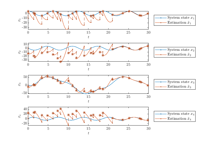
Example Output
The solution to the estimation over network system from \(z(0,0)=[1, 0.1, 1, 0.6]^\top, \hat{z}(0,0)=[-10, 0.5, 0, 0, 0]^\top\) , u(t)=50*sin(0.1*t),and with T=30 , J=100 , rule=1 shows that the estimated state approaches the system's state before \(t = T\) , with a small error.
References
[1] F. Ferrante, F. Gouaisbaut, R. G. Sanfelice, and S. Tarbouriech. State estimation of linear systems in the presence of sporadic measurements. Automatica, 73:101–109, November 2016.