Introduction to the Simulink-based Hybrid Equation Simulator
This document describes the Simulink-based hybrid equation simulator from the Hybrid Equations Toolbox, including an introduction to the primary components. For documentation regarding cyber-physical components, see here . A list of examples are available here . For a description of the internal workings of Hybrid System blocks, see The Integrator System .
Contents
- Primary Components
- Deciding Whether to Use Embedded or External Functions
- How to Use a Hybrid System Block
- Writing Functions for \(f\) , \(g\) , \(C\) , and \(D\)
- Defining Function Parameters
- Variable Initialization
- Postprocessing and Plotting solutions
- Automatically Running Initialization and Postprocessing Scripts
Primary Components
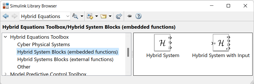
The HyEQ Toolbox includes four main Simulink library blocks that allow for simulation of hybrid systems:
- \(\mathcal{H}\) defined with external functions . For this block, the data of the system \((C, f, D, g)\) are defined as MATLAB functions in plain-text .m files. This block does not support systems with inputs.
- \(\mathcal{H}\) defined with external functions and inputs . This block is the same as the prior one, except that it has inputs.
- \(\mathcal{H}\) defined with embedded functions . For this block, the data of the system \((C, f, D, g)\) are defined as embedded functions that can only be edited within Simulink. This block does not support systems with inputs.
- \(\mathcal{H}\) defined with embedded functions and inputs . This block is the same as the prior one, except that it has inputs.
The following image shows these blocks in the Simulink Library Browser.

Next, we see inside the Simulink blocks for simulating a hybrid system \(\mathcal{H}\) with inputs implemented with using embedded MATLAB function blocks .
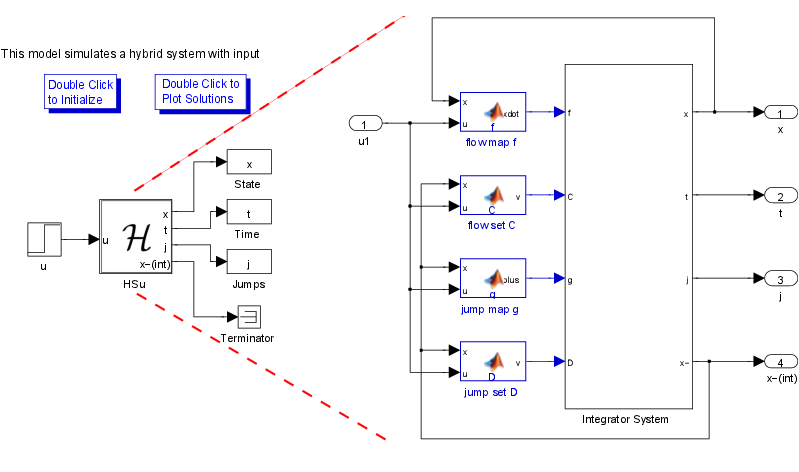
In this implementation, four blocks are used to define the data of the hybrid system \(\mathcal{H}\) :
- The flow map is implemented in the embedded function block flow map f . Its input is a vector with components defining the state of the system \(x\) , and the input \(u\) . Its output is the value of the flow map \(f\) which is connected to the input of an integrator.
- The flow set is implemented in the embedded function block flow set C . Its input is a vector with components \(x^-\) and input \(u\) of the Integrator system . Its output is equal to \(1\) if the state belongs to the set \(C\) or equal to \(0\) otherwise. The minus notation denotes the previous value of the variables (before integration). The value \(x^-\) is obtained from the state port of the integrator.
- The jump map is implemented in the embedded function block jump map g . Its input is a vector with components \(x^-\) and input \(u\) of the Integrator system . Its output is the value of the jump map \(g\) .
- The jump set is implemented in the embedded function block jump set D . Its input is a vector with components \(x^-\) and input \(u\) of the Integrator system . Its output is equal to \(1\) if the state belongs to \(D\) or equal to \(0\) otherwise.
Deciding Whether to Use Embedded or External Functions
Prior to v3.0, only hybrid systems with embedded function blocks could be used to model systems with inputs, but now external functions can be used for systems with inputs as well. Thus, embedded vs. external functions are interchangable in terms of the types of systems they can model. There are other benefits and limitations to each, however.
External functions have the benefits that the functions are stored in plaintext .m files, so they can be easily tracked with source control managagment software, such as Git. They can also be resused without modification when using the HyEQ MATLAB library.
Embedded functions, on the other hand, result in the entire Simulink model being self-contained in a single file. Simulations may also be somewhat faster and can be compiled and deployed to embedded systems. The code used in an embedded function is restricted to MATLAB Language Features Supported for C/C++ Code Generation .
How to Use a Hybrid System Block
To add a Hybrid System to a Simulink model:
- Open the Simulink Library Browser and select "Hybrid Equations Toolbox" from the list of toolboxs and drag the desired block into your model.
- Double-click on the Hybrid System block to open a dialog box. Fill each field with either your desired value or a variable that you define in the initialization script.
- Define the functions for \(f\) , \(g\) , \(C\) , and \(D\) for the hybrid system. The process for specifying the functions are different for embedded vs. external functions, so we describe each approach below.
-
Connect the intputs and outputs as desired. For Hybrid System blocks with inputs, there are two state outputs
\(x\)
and
\(x^-\)
. Most of the time, you should use the
\(x\)
output, as it is the current state of the Hybrid Subsystem block. Sometimes, however, when you have a closed loop system, Simulink warns of an "
- When a HyEQ block is added to a Simulink model, several things are changed in the model. In particular, solver settings are changed such that the relative tolerance is a variable named RelTol , the maximum step is MaxStep , and the simulation stop time is T . You must define RelTol , MaxStep , and T prior to running the Simulink model (e.g., in an initialization script, as described below).
How to define \(f\) , \(g\) , \(C\) , and \(D\) in hybrid systems with external functions . To specify \(f\) , \(g\) , \(C\) , and \(D\) for a hybrid system with external functions block, create four MATLAB function files (.m extensions) that are either on the MATLAB path or in the working directory from which you will run the Simulink model. (Using packages can help prevent name conflicts.) Then, enter the name of each function preceded by an @ sign in the corresponding field in the mask dialog. For example, if the flow map function is placed in a function file name f.m , then the Flow Map field in the mask dialog should contain "@f" (without quotation marks).
As an alternative to creating function files, you can write anonymous functions , such as
@(x, u, parameters) parameters.A*x + parameters.B*u
directly into any of the function handle fields in the mask dialog.
How to define \(f\) , \(g\) , \(C\) , and \(D\) in hybrid systems with embedded functions . To specify \(f\) , \(g\) , \(C\) , and \(D\) for a Hybrid System with Embedded Functions block, "Look inside" the block mask by either clicking the down arrow in the lower-left corner or selecting "Mask" > "Look Under Mask" from the context menu. Double-click on each MATLAB Function block to edit the respective functions. (There's nothing "magic" about the MATLAB function blocks. If desired, these blocks can be replaced with any other Simulink blocks that have the correct input and output dimensions.)
Writing Functions for \(f\) , \(g\) , \(C\) , and \(D\)
Regardless of whether you are using a Hybrid System block with embedded or external functions, the definitions of \(f\) , \(g\) , \(C\) , and \(D\) follow the same form. When creating a system without inputs, each function must take two input arguments: the state "x" and parameters object "parameters". (The "parameters" argument is described later.) When creating a system with inputs, each function must, instead, have three input arguments: the state "x", the input "u", and a parameter object "parameters".
For both systems with and without inputs, each function must have a single output argument. For f and g , the output is a column vector that matches the size of "x". For C and D , the output is scalar that takes values in \(\{\texttt{0}, \texttt{1}\}\) .
Thus, example function signatures for systems without inputs are as follow:
function xdot = f(x, parameters)
function inC = C(x, parameters)
function xplus = g(x, parameters)
function inD = D(x, parameters)
For systems with inputs, the following function signatures can be used:
function xdot = f(x, u, parameters)
function inC = C(x, u, parameters)
function xplus = g(x, u, parameters)
function inD = D(x, u, parameters)
The names of the functions and arguments can be modified when using external functions, but for embedded functions the input arguments must match those given above (unless the names of the data signals are renamed in the Ports and Data Manager ).
Defining Function Parameters
Often, in addition to the state and input, the values return by f , g , C , and D will depend on some constants. For example, the flow map of the bouncing ball depends on the rate of acceleration due to gravity. One could simply define
g = -9.8;
within the function, but this is bad practice. What will you do, for instance, if you want to sometimes simulate a bouncing ball on the Moon instead, where gravity is weaker? You would need to modify the function each time you change g . To avoid this, a parameters object, defined by the user, is given as the last input argument for each function. The parameters object can be any type of MATLAB object (e.g., an array or object), but the recommended approach is to use a struct because it allows new parameters to be added easily and makes the code easy to read. In an initialization script, a parameters struct can be created as follows:
parameters = struct();
parameters.A = [0, 1; 0, 0];
parameters.B = [0; 1];
parameters.optimizer = 'BFGS'; % Nonnumeric values are OK.
The parameters struct is passed to a hybrid system block by entering the name of the variable in the "Parameters" field of the mask dialog.
Then, within f , g , C , and D , parameters are accessed via the last input argument, as shown below.
function xdot = f(x, u, parameters)
    % Flow map
    A = parameters.A;
    B = parameters.B;
    xdot = A*x + B*u;
end
The last input argument parameters must be present (even if it is unused). For embedded functions, its name must be "parameters" (MATLAB may suggest replacing it with "~" if it is unused, but this will cause an error).
WARNING: The parameters object should be constant while simulating a hybrid system. Modifying parameters within f , g , etc., could produce unpredictable behavior because the hybrid solver sometimes backtracks in time (e.g., when searching for the time when a jump occurs). Therefore, all values that change during a solution must be included in the state vector x .
Variable Initialization
Before a Simulink model is run, all variables referenced in block parameters or the model configuration parameters must be defined in the MATLAB workspace. This can be done by entering the variables one-by-one in the MATLAB command window, but for the sake of quickly, easily, and accurately reproducing results, it is best to put the variable definitions into an initialization script. In this documentation we refer to the initialzation script as initialize.m .
Within initialize.m , it is typically necessary to define the following:
- Initial conditions (e.g., x0 , z0 , etc.)
- Parameter objects, as described above
- The maximum flow time T
- The maximum number of jumps J
- The relative error tolerance RelTol
- The maximum integration step size MaxStep .
The following initialization script is used for the bouncing ball model .
% Initialization script for Bouncing Ball example.

% Initial conditions
x0 = [1; 0];

% Physical variables
parameters = struct();
parameters.gamma = -9.81; % Acceleration due to gravity.
parameters.lambda = 0.9;  % Coefficient of restitution.

% Simulation horizon
T = 10;
J = 30;

% Solver tolerances
RelTol = 1e-6;
MaxStep = 1e-2;
We define the values of RelTol and MaxStep because the default integration settings do not always produce simulations with the desired accuracy or speed. See odeset for a description of RelTol , MaxStep , and other solver settings. These parameters can have significant effects on the speed and accuracy of solutions. To modify other solver settings, open Modeling>Model Settings>Solver .
The name T should be used for the maximum flow time because the simulation stop time is automatically set to T whenever a HyEQ block is added to a model. Other variables names, however, such as x0 , J , and parameters , can be changed on a block-by-block basis so long as the names are consistent between the fields in the block mask dialogs and in the initialization script.
After initialization, the simulation is run by clicking the run button or selecting Simulation>Start .
Postprocessing and Plotting solutions
Similarly to the initialization script, a postprocessing script, which we will call postprocess.m , here, is used to generate plots of solutions after the simulation is run. Below is an example of postprocess.m for the bouncing ball example. The functions used to generate the plots are described in Creating plots with HybridPlotBuilder .
%% Postprocessing script for Bouncing Ball example.

% Construct a HybridArc object from (t, j, x) computed by Simulink so that
% we can use the plotting tools associated with HybridArcs, namely
% HybridPlotBuilder.
sol = HybridArc(t, j, x);

% Plot the solution vs. t.
figure(1)
clf
plotFlows(sol)

% Plot the solution in the phase plane.
figure(2)
clf
plotPhase(sol)
grid on

% Plot the first component of the solution vs. t and j.
figure(3)
clf
plotHybrid(sol.select(1))
grid on
view(37.5,30)
Automatically Running Initialization and Postprocessing Scripts
The scripts initialize.m and postprocess.m , described above, can be run manually in the MATLAB editor or command window, but to run them automatically use model callbacks . To setup model callbacks, open the Simulink Library Browser and navigate to Hybrid Equations Toolbox > Other.
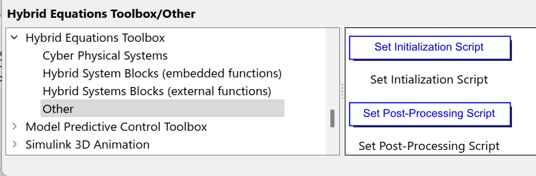
Then, drag the "Set Initialization Script" and "Set Post-Processing Script" blocks to your model and double click on them. A file selection dialog will open that allows you to select a MATLAB .m script file to use in the callback. After a callback script is set, the "Set Initialization Script" and "Set Post-Processing Script" blocks can be deleted from your model.
To define model callbacks manually or remove existing callbacks:
- open the "Modeling" tab in Simulink
- open the "Modeling Setup" menu
- open "Model Properties"
- open the "Callbacks" tab.
Use the InitFcn callback to specify code to run before the Simulink model starts and StopFcn to specify code to run after the model finishes. Typically, the InitFcn callback contains code that calls an initialization script, such as
initialize;
and the StopFcn callback calls a post-processing script, such as
postprocess;