Example 1: Vehicle on Path with Boundaries
In this example, a vehicle is controlled such that it moves along a path.
Contents
The files for this example are found in the package hybrid.examples.vehicle_on_constrained_path :
- initialize.m
- vehicle_on_path.slx
- postprocess.m
The contents of this package are located in Examples\+hybrid\+examples\vehicle_on_constrained_path (clicking this link changes your working directory).
Consider a vehicle modeled by a Dubins vehicle model with state vector \(x=[\xi_1, \xi_2, \xi_3]^\top\) and with dynamics given by \(\dot{\xi_1}=u\cos{\xi_3}\) , \(\dot{\xi_2}=u\sin{\xi_3}\) , and \(\dot{\xi_3}=-\xi_3+r(q)\) . The input \(u\) is the tangential velocity of the vehicle, \(\xi_1\) and \(\xi_2\) describe the vehicle's position on the plane, and \(\xi_3\) is the vehicle's orientation angle. Also consider a switching controller attempting to keep the vehicle inside the boundaries of a track given by \(\{(\xi_1,\xi_2):-1\leq\xi_1\leq1\}\) . A state \(q \in \{1,2\}\) is used to define the modes of operation of the controller. When \(q=1\) , the vehicle is traveling to the left, and when \(q=2\) , the vehicle is traveling to the right. A logic variable \(r\) is defined in order to steer the vehicle back inside the boundary. The state of the closed-loop system is given by \(x := [\xi^\top\ q]^\top\) .
Mathematical Model
A model of such a closed-loop system is given by
\[ \begin{array}{l} f(x,u) := \left[\begin{array}{c} u\cos(\xi_3) \\ u\sin(\xi_3)\\ -\xi_3+r(q) \\ 0 \end{array}\right] + \left[\begin{array}{c} 0 \\ 0 \\ 0 \\ 1 \end{array}\right] u, \quad r(q) := \left\{\begin{array}{cc} \frac{3\pi}{4} & \textrm{if } q=1 \\ \frac{\pi}{4} & \textrm{if } q=2 \\ \end{array}\right. \\ \\ C := \{(\xi, q, u)\in \mathbb{R}^{3}\times\{1,2\}\times \mathbb{R}\mid (\xi_1 \leq 1,\ q = 2) \textrm{ or } (\xi_1 \geq -1,\ q=1)\}, \\ \\ g(x,u) := \left\{\begin{array}{ll} \left[\begin{array}{c} \xi \\ 2 \end{array}\right] & \textrm{if } \xi_1\leq-1,\ q=1 \\ \\ \left[\begin{array}{c} \xi \\ 1 \end{array}\right] & \textrm{if } \xi_1\geq 1,\ q=2, \end{array} \right. \\ \\ D := \{(\xi, q, u)\in \mathbb{R}^{3}\times\{1,2\} \times \mathbb{R} \mid(\xi_1 \geq 1,\ q = 2) \textrm{ or } (\xi_1 \leq -1,\ q=1)\} \end{array}\]
Simulink Model
The Simulink blocks for the hybrid system in this example are included below.
flow map f block
function xdot = f(x, u)
    % Flow map for Vehicle Traveling on a Track

    % State
    xi3 = x(3); % Orientation angle
    q = x(4);

    % q = 1 --> going left
    % q = 2 --> going right
    if q == 1
        r = 3*pi/4;
    elseif q == 2
        r = pi/4;
    else
        r = 0;
    end

    xi1dot = u*cos(xi3);  % Tangential velocity in x-direction
    xi2dot = u*sin(xi3);  % Tangential velocity in y-direction
    xi3dot = -xi3 + r;    % Angular velocity
    qdot = 0;

    xdot = [xi1dot; xi2dot; xi3dot; qdot];
end
flow set C block
function inC  = C(x, u)
    % Flow set for Vehicle Traveling on a Track

    % State
    xi1 = x(1);      %x-position
    q = x(4);

    % q = 1 --> going left
    % q = 2 --> going right
    if ((xi1 < 1) && (q == 2)) || ((xi1 > -1) && (q == 1))  % flow condition
        inC = 1;  % report flow
    else
        inC = 0;   % do not report flow
    end
end
jump map g block
function xplus = g(x, u)
    % Jump map for Vehicle Traveling on a Track

    % State
    xi = x(1:3);

    % q = 1 --> going left
    % q = 2 --> going right
    q = x(4);

    if ((xi(1) >= 1) && (q == 2)) || ((xi(1) <= -1) && (q == 1))
       qplus = 3-q;
    else
        qplus = q;
    end

    xplus = [xi; qplus];
end
jump set D block
function inD  = D(x, u)
    % Jump set indicator function for Vehicle Traveling on a Track

    % State
    xi1 = x(1);      %x-position

    % q = 1 --> going left
    % q = 2 --> going right
    q = x(4);

    if ((xi1 >= 1) && (q == 2)) || ((xi1 <= -1) && (q == 1))  % jump condition
        inD = 1;  % report jump
    else
        inD = 0; % do not report jump
    end
end
Example Output
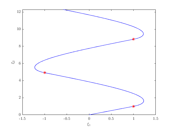
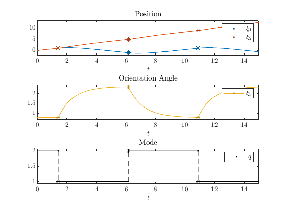
A solution to the system above is plotted below with initial position \((\xi_1,\xi_2)=(0,0)\) , initial orientation angle \(\xi_3=\frac{\pi}{4}\) radians, T=15 , J=10 , and rule=1 .
The following plot depicts the trajectory of the vehicle.