CPS Component: Zero-Order Hold (ZOH)
A zero-order hold (ZOH) converts a digital signal at its input into an analog signal at its output. Its output is updated at discrete time instants, typically periodically, and held constant in between updates, until new information is available at the next sampling time. In this example, a ZOH model is modeled in Simulink as a hybrid system with an input, where the input is the signal to sample.
Contents
The files for this example are found in the package hybrid.examples.zero_order_hold :
- initialize.m
- zoh.slx
- postprocess.m
The contents of this package are located in Examples\+hybrid\+examples\zero_order_hold (clicking this link changes your working directory).
Mathematical Model
The ZOH system is modeled as a hybrid system with the following data:
\[\begin{array}{ll} f(q,u):=\left[\begin{array}{c} 0 \\ 0 \\ 1 \end{array}\right], & C := \{ (x,u) \mid \tau\in [0, T^{*}_{s}] \} \\ \\ g(x,u):= \left[ \begin{array}{c} u \\ 0 \end{array}\right], & D: = \{ (x,u) \mid \tau_{s} \geq T^{*}_{s}\} \end{array}\]
\[ y = h(x) := x \]
where the input and the state are given by \(u \in \mathbb{R}^{2}\) , and \(x = (m_{s}, \tau_{s})\in \mathbb{R}\times \mathbb{R}^{2}\) , respectively.
Steps to Run Model
The following procedure is used to simulate this example using the model in the file zoh.slx :
- Open zoh.slx in Simulink (clicking this link changes your working directory and opens the model).
- Double-click the block labeled Double Click to Initialize .
- To start the simulation, click the run button or select Simulation>Run .
- Once the simulation finishes, click the block labeled Double Click to Plot Solutions . Several plots of the computed solution will open.
Simulink Model
The following diagram shows the Simulink model of the ZOH. When the Simulink model is open, the blocks can be viewed and modified by double clicking on them. To look inside the ZOH block, click the down arrow in the lower-left corner of the block or open the block's context menu and select Mask > Look under mask.
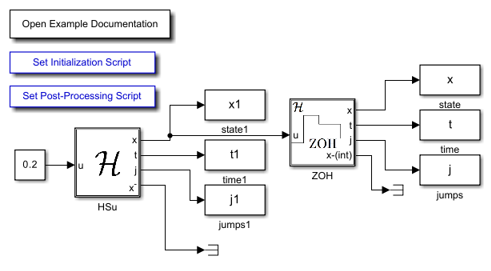
The functions used to define \((f, g, C, D)\) within the ZOH block are included below.
flow map f block
function xdot = f(x, vs)
    % Flow map for zero-order hold.
    tau_dot = 1;
    xdot = zeros(size(x)); % All entries zero, except tau_dot
    xdot(end) = tau_dot;
end
flow set C block
function inC  = C(x, vs, sample_time)
    % Flow set indicator function zero-order hold.
    tau = x(end); % Timer state
    if tau>=0 && tau <= sample_time
        inC = 1; % report flow
    elseif tau > sample_time
        inC = 0; % do not report flow
    else
        inC = 0;
    end
end
jump map g block
function xplus = g(x, vs)
    % Jump map for zero-order hold.
    msplus = vs; % output = measured input
    tau_splus = 0; % Timer tau_s
    xplus = [msplus; tau_splus];
end
jump set D block
function inD  = D(x, vs, sample_time)
    % Jump set indicator function for zero-order hold.
    tau_s = x(end); % timer state
    if tau_s>=0 && tau_s<= sample_time
        inD = 0; % do not report jump
    elseif tau_s> sample_time
        inD = 1; % report jump
    else
        inD = 0;
    end
end
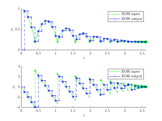
Example Output
In this example, a signal is generated by the bouncing ball system with the height of the platorm chosen to be constant, equal to \(0.2\) . The signal is then passed through a ZOH block. The initial state of the bouncing ball system is \([1, 0]^\top\) . The solution to the ZOH system from \(x(0,0)=[1, 0, 0]^\top\) and with T=10 , J=100 , rule=1 shows the output signal after the ZOH process.