Creating and Simulating Multiple Interlinked Hybrid Systems

In this document, we demonstrate how to simulate multiple interlinked hybrid systems using the CompositeHybridSystem class.

Mathematical Formulation
Outline of How To Create a Composite System
Creating Subsystems
Output Functions
Defining HybridSubsystems In-Line
Creating a Compositite Hybrid System from Multiple Subsystems
Subsystem Identifiers
Input Functions
Computing Solutions
Plotting Solutions
Subsystem Solutions
Plotting Input and Output Signals
Example: Single Subsystem

Mathematical Formulation

Consider the controlled hybrid systems \(\mathcal H_1\) and \(\mathcal H_2\) with data \((f_1, g_1, C_1, D_1)\) and \((f_2, g_2, C_2, D_2)\) and state spaces \(\mathcal X_1\) and \(\mathcal X_2.\) Let \(x_1 \in \mathcal X_1\) and \(x_2 \in \mathcal X_2.\) The dynamics of \(\mathcal H_1\) and \(\mathcal H_2\) are

\[ \left\{\begin{array}{ll} \dot{x}_1 = f_1(x_1, u_{C1}, t, j_1) &(x_1, u_{C1}, t, j_1) \in C_1 \\ x_1^+ = g_1(x_1, u_{D1}, t, j_1) &(x_1, u_{D1}, t, j_1) \in D_1 \end{array} \right. \quad \]

Each subsystem also has output values

\[ \left\{\begin{array}{l} y_{C1} = h_{C1}(x_1, u_{C1}, t, j_1) \\ y_{D1} = h_{D1}(x_1, u_{D1}, t, j_1) \end{array} \right. \quad \]

Note that \(\mathcal H_1\) and \(\mathcal H_2\) use the same continuous time \(t\) but different discrete times \(j_1\) and \(j_2\) because they jump independently of each other.

To create feedback connections between \(\mathcal H_1\) and \(\mathcal H_2,\) we choose the inputs

\[ \left\{\begin{array}{l} u_{C1} = \kappa_{1C}(y_{C1}, y_{C2}, t, j_1) \\ u_{D1} = \kappa_{1D}(y_{D1}, y_{D2}, t, j_1)\end{array}\right.\quad \]

We define the system \(\tilde H\) as the composition of subsystems \(\mathcal H_1\) and \(\mathcal H_2.\) The state \(\tilde x\) of \(\tilde H\) is the concatenation of \(x_1\) and \(x_2\) along with \(j_1, j_2\in N\) that track the discrete times of the subsystems (since they can jump at different times). That is, \(\tilde x = (x_1, x_2, j_1, j_2).\) The system will flow when both subsystems are in their respective flow sets and to jump whenever either is in their jump set. Thus, we use the flow set \(\tilde C := C_1 \times C_2,\) and the jump set \(\tilde D = (D_1 \times \mathcal X_2) \bigcup (\mathcal X_1 \times D_2).\) In simulations, priority is given to jumps when \(x\) in the intesection of \(C\) and \(D\) . The flow map is

\[ \dot{\tilde{x}} = \tilde{f}(\tilde x):= \left[\begin{array}{c} f_1(x_1, u_{1C}, t, j_1) \\ f_2(x_2, _{2C}, t, j_2) \\ 0 \\ 0 \end{array}\right].\]

The jump map depends on whether \(\tilde x\) is in \(D_1\times \mathcal X_2\) or \(\mathcal X_1 \times D_2\) . If \(\tilde x \in D_1\times \mathcal X_2,\) then

\[\tilde x^+ = \tilde{g}_1(\tilde x):= \left[\begin{array}{c} g_1(x_1, u_{1D}, t, j_1) \\ x_2 \\ j_1 + 1 \\ j_2 \end{array}\right],\]

if \(\tilde x \in \mathcal X_1 \times D_2,\) then

\[\tilde x^+ = \tilde{g}_2(\tilde x):= \left[\begin{array}{c} x_1 \\ g_2(x_2, u_{2D}, t, j_2) \\ j_1 \\ j_2 + 1 \end{array}\right],\]

and if \(\tilde x \in D_1 \times D_2,\) then

\[\tilde x^+ = \tilde{g}_2(\tilde x):= \left[\begin{array}{c} g_1(x_1, u_{1D}, t, j_1) \\ g_2(x_2, u_{2D}, t, j_2) \\ j_1 + 1\\ j_2 + 1 \end{array}\right].\]

Outline of How To Create a Composite System

To implement a composite hyrbid system, we use the CompositeHybridSystem and HybridSubsytem classes. Each CompositeHybridSystem contains one or more HybridSubsystem objects. The following diagram shows the relationship between classes. An open arrowhead indicates a subclass/superclass relationship. (Note that HybridSubsystem is not a subclass of HybridSystem .)

Implementing a composite system consists of three steps:

Create one or more HybridSubsystem objects, either by writing custom subclasses or using existing classes (such as those in hybrid.subsystems ).
Create a CompositeHybridSystem from the collection of HybridSubsystem objets.
Define input functions for each subsystem.

A solution to a CompositeHybridSystem can be computed and plotted just like any other HybridSystem object. Information about subsystem state, input, and output values are also provided.

Creating Subsystems

In the Hybrid Equations Toolbox, hybrid subsystems, such as \(\mathcal{H}_1\) and \(\mathcal{H}_2\) above, are represented by the HybridSubsystem class. HybridSubsystem is an abstract class, which means that some of its methods are not fully defined, so a HybridSubsystem object cannot be created directly. Instead, it is necessary to implement a subclass of HybridSubsystem (or use an existing subclass) that provides the full definitions of the abstract methods in HybridSubsystem . In this tutorial, we use several HybridSubsystem subclasses located in the hybrid.subsystems package.

help hybrid.subsystems

Contents of hybrid.subsystems package:

          ContinuousSubsystem - Hybrid subsystems that do not have discrete dynamics.
ControllerWithComputationTime - Create a HybridSubsystem that computes a control law with a delayed
    LinearContinuousSubsystem - Hybrid subsystems that have linear continuous dynamics and no discrete dynamics.
          MemorylessSubsystem - Hybrid subsystems with output that is generated solely from the input (no state values).
          OutputMemoizorMixin - hybrid.subsystems.OutputMemoizorMixin is a class.
              SwitchSubsystem - Hybrid subsystems for switching the output between two input values. (EXPERIMENTAL)
                ZeroOrderHold - Hybrid subsystems that periodically sample the input to generate a piecewise constant output.
              function_handle - hybrid.subsystems.function_handle is a class.

See here for details regarding namespace packages.

We will look at hybrid.examples.BouncingBallSubsystem as an example of how to implement a HybridSubsystem . A script for running this example is provided at hybrid.examples.run_bouncing_ball_with_input (the prefix hybrid.examples. indicates the package namespace that contains BouncingBallSubsystem.m and run_bouncing_ball_with_input.m ). Mathematically, we write the hybrid subsystem as

\[ \mathcal{H}_{\mathrm{BB}}:\left\{\begin{array}{ll} \dot{x} = f_{\mathrm{BB}}(x) := \left[\matrix{x_2 \\ -\gamma}\right] & x \in C_{\mathrm{BB}} := \{(x_1, x_2) \in R^2 \mid x_1 \geq 0 \textrm{ or } x_2 \geq 0\} \\ x^+ = g_{\mathrm{BB}}(x, u_{D}) := \left[\matrix{x_1 \\ -\lambda x_2}\right] + \left[\matrix{0 \\ 1}\right]u_D & x \in D_{\mathrm{BB}} := \{(x_1, x_2) \in R^2 \mid x_1 \leq 0, x_2 \leq 0\} \end{array} \right.\]

The bouncing ball subsystem is translated into MATLAB code as follows.

classdef BouncingBallSubsystem < HybridSubsystem
% A bouncing ball with an input modeled as a HybridSubsystem subclass.


    % Define properties of the system that can be modified.
    properties
        gamma = -9.8; % Acceleration due to gravity.
        lambda = 0.9; % Coefficient of bounce restitution.
    end

    % Define properties of the system that cannot be modified (i.e., "immutable").
    properties(SetAccess = immutable)
        % The index of the ball's height within the state vector.
        height_index = 1;
        % The index of the ball's velocity within the state vector.
        velocity_index = 2;
    end
    
    methods
        function obj = BouncingBallSubsystem() % Constructor.
            state_dim = 2;
            input_dim = 1;
            output_dim = 2; % Matches state_dim (default).
            output_fnc = @(x) x; % Full-state output (default).

            % Call the constructor of the superclass 'HybridSubsystem' to create
            % the object.
            obj = obj@HybridSubsystem(state_dim, input_dim, output_dim, output_fnc);
        end

        % To define the data (f, g, C, D) of the system, we implement 
        % the abstract functions from HybridSubsystem.m
        
        function xdot = flowMap(this, x, u, t, j)  
            % Extract the state component 'v'.
            v = x(this.velocity_index);

            % Define the value of f(x, u). 
            xdot = [v; this.gamma];
        end

        function xplus = jumpMap(this, x, u, t, j) 
            % Extract the state components.
            h = x(this.height_index);
            v = x(this.velocity_index);
            % Define the value of g(x, u). 
            xplus = [h; -this.lambda*v + u];
        end 

        function inC = flowSetIndicator(this, x, u, t, j)
            % Extract the state components.
            h = x(this.height_index);
            v = x(this.velocity_index);

            % Set 'inC' to 1 if 'x' is in the flow set and to 0 otherwise.
            inC = h >= 0 || v >= 0;
        end 

        function inD = jumpSetIndicator(this, x, u, t, j)
            % Extract the state components.
            h = x(this.height_index);
            v = x(this.velocity_index);

            % Set 'inD' to 1 if 'x' is in the jump set and to 0 otherwise.
            inD = h <= 0 && v <= 0;
        end
    end
end

In the constructor for BouncingBallSubsystem , the state, input, and output dimensions and the output function are set by passing values to the superclass constructor obj@HybridSubsystem . The flowMap , jumpMap , flowSetIndicator , and jumpSetIndicator functions are defined similarly to the corresponding functions in HybridSystem classes with two exceptions:

The subsystem input \(u\) is included as the second input argument for each functions.
All four input arguments (i.e., 'x, u, t, j' ) must be included, even if they are unused. (Unused arguments can be replaced with '~' .)

Output Functions

For each subsystem, the flow output function \(h_C\) and a jump output function \(h_D\) can be set by passing zero, one, or two function handles to the HybridSubsystem superclass constructor. If no output functions handles are given, explictly, then the output functions return the full subsystem state \(h_C(x) = h_D(x) = x\) . If one function handle is given, then it defines output for both flows and jumps. If two functions are given, then the first defines flow output and the second defines jump output. Both functions must have the same size outputs, which match the output_dimension. The output function handle must have input arguments in one of the following forms: (x), (x, u), (x, u, t) , or (x, u, t, j) . In order for the solver to determine the order to evaluate input and outputs, the u input argument must be omitted or replaced with '~' if it is unused.

Defining HybridSubsystems In-Line

As an alternative to writing new HybridSubsystem subclasses, the HybridSubsystemBuilder class can be used to create HyrbidSubsystems in-line (see doc HybridSubsystemBuilder for details).

HybridSubsystemBuilder()...
    .stateDimension(2)...
    .inputDimension(1)...
    .outputDimension(1)...
    .flowMap(@(x, u) x + [1; 0]*u)...
    .jumpMap(@(x) 0.5*x)...
    .flowSetIndicator(@(x) norm(x) <= 0)...
    .jumpSetIndicator(@(x) norm(x) >= 0)...
    .flowOutput(@(x) x(1))...
    .jumpOutput(@(x) x(2))...
    .build();

Creating subsytems with HybridSubsystemBuilder is not recommended except for prototypes or demonstrations (such as this tutorial) becuase it makes code execution slower and dubugging more difficult.

Creating a Compositite Hybrid System from Multiple Subsystems

In this example, two subsystems are created. The first is a bouncing ball with controlled impulses applied at each bounce.

ball_subsys = hybrid.examples.BouncingBallSubsystem();

The second subsystem is a controller that decides the strength of each impluse with the goal of achieving periodic bouncing. The control strategy is very simple. At each bounce, the controller resets a timer. If the timer at the next bounce is less than the target period, then the strength of the impulse is increased, and if it is less, then the impulse is decreased. The state of the controller is \((p, \tau)\) where \(p\) is the strength of the impulse that will be applied at the next jump and \(\tau\) is the timer. Let \(T\) be the desired period. Then, the dynamics of the controller are chosen to be

\[\left\{ \begin{array}{ll} \left[\matrix{ \dot p \\ \dot \tau } \right] = \left[\matrix{0 \\ 1}\right] & u \in C := \{0\} \\ \left[\matrix{p^+ \\ \tau^+ } \right] = \left[\matrix{\max\{0, p + (T-\tau)\} \\ 0}\right] & u \in D := \{1\} \end{array} \right. .\]

target_period = 2.0;

% For clarity, we name the indices for each component in the state vector.
p_ndx = 1;
tau_ndx = 2;

% During flows, p is constant and tau increases at a constant rate.
f = @(x) [0; 1]; % pdot = 0, taudot = 1.

% At each jump, the controller updates the first component based on whether the
% timer was more or less than the target period.
g = @(x, u) [max(0, x(p_ndx) + target_period-x(tau_ndx)); 0];

controller_subsys = HybridSubsystemBuilder()...
                    .stateDimension(2)... % state: p and \tau
                    .inputDimension(1)... % input: u=1 if ball should bounce and 0 otherwise.
                    .outputDimension(1)... % output: impulse p
                    .flowMap(f)...
                    .jumpMap(g)...
                    .flowSetIndicator(@(x) 1)...
                    .jumpSetIndicator(@(~, u) u)... % 'u' will be 1 when the ball bounces.
                    .output(@(x) x(p_ndx))... % Output 'p'
                    .build();

We can test that the data for the subsystems return values of the correct sizes and assert whether particular points are inside \(C\) or \(D\) .

 % Evaluates functions at origin and checks output sizes.
ball_subsys.checkFunctions();

% Evaluate functions at x=[10;0] and check output sizes.
ball_subsys.checkFunctions([10; 0]);

% Above ground.
ball_subsys.assertInC([1; 0]);
ball_subsys.assertNotInD([1; 0]);

% At ground, stationary.
ball_subsys.assertInC([0; 0]);
ball_subsys.assertInD([0; 0]);

% Below ground, moving down.
ball_subsys.assertNotInC([-1; -1]);
ball_subsys.assertInD([-1; -1]);
disp('All checks passed.')

All checks passed.

Now that we have two subsystems, we pass these to the CompositeHybridSystem constructor to create a coupled system. There are two forms of the constructor arguments. The first is to simply pass the list of subsystems.

sys = CompositeHybridSystem(bb_plant, bb_controller);

Alternatively, names can be given to each subsystem by passing strings before each subsystem in the CompositeHybridSystem constructor. If any subsystems are named, then all the subsystems must be named.

sys_bb = CompositeHybridSystem('Ball', ball_subsys, 'Controller', controller_subsys)

sys_bb = 
CompositeHybridSystem:
├ Subsystem 1: 'Ball' (hybrid.examples.BouncingBallSubsystem)
│ 		  Flow input: @(~,~,~)zeros(1,1)
│ 		  Jump input: @(~,~,~)zeros(1,1)
│ 		      Output: y1=@(x)x
│ 		 Dimensions: State=2, Input=1, Output=2
└ Subsystem 2: 'Controller' (hybrid.internal.EZHybridSubsystem)
  		  Flow input: @(~,~,~)zeros(1,1)
  		  Jump input: @(~,~,~)zeros(1,1)
  		      Output: y2=@(x)x(p_ndx)
  		 Dimensions: State=2, Input=1, Output=1

Subsystem Identifiers

For each subsystem, we define its subsystem identifiers as the following:

The positive integer matching the ordinal position of the subsystem in the CompositeHybridSystem constructor arguments.
A refernce to the HybridSubsystem object itself (such as the variables ball_subsys and controller_subsys , above).
The subsystem's name, if given in the constructor.

For example, for the system constructed above, the subsystem identifiers for each subsystem are:

1 , ball_subsys , and 'Ball' .
2 , controller_subsys , and 'Controller' .

Input Functions

Each subsystem has a flow input function and a jump input function. The flow input function determines the input values for the subsystem during each interval of flow and the jump input function determines the input at each jump. The functions setFlowInput , and setJumpInput set the respective input functions for a given subsystem and setInput sets both the flow input and the jump input to a single function. The first argument is a subsystem identifier, described above. The second argument is the input function, given as a function handle. The input function must have one of the following forms:

@()
@(y1)
\(\vdots\)
@(y1, y2, ..., yN)
@(y1, y2, ..., yN, t)
@(y1, y2, ..., yN, t, j) where '...' is replaced with the appropriate number of arguments.

sys.setJumpInput(1, @(y1, y2) y2);
sys.setInput(bb_controller, @(y1, y2) y2);
sys.setFlowInput('Plant', @(y1, y2) y1(1)-y2(1));

The input functions must have between zero and \(N+2\) input arguments, where \(N\) is the number of subsystems. The first \(N\) arguments are passed the output values of each corresponding subsystem, and, if present, the \(N+1\) argument is passed the continuous time t for the composite system (which equals the continuous time of the subsystems), and the \(N+2\) argument is passed the discrete time j for that subsystem, which is not (in general) the same as the discrete time of the composite system.

As with output functions, any unused input arguments (especially the inputs that recieve outputs from other systems, e.g., y1 , y2 , etc.) should be omitted or replaced with '~' so that the solver can determine which order to evaluate the input and output functions.

For our example, we set the jump input for the ball such that the output of the controller is passed as the input to the ball.

sys_bb.setJumpInput('Ball',  @( ~, y_controller) y_controller);

The input for the controller is set such that the output of the ball's jumpSetIndicator is passed to the input of the controller. Thus, the input to the controller is 1 if the ball should jump and 0 otherwise. This allows the controller to know when the ball hits the ground.

controller_fcn = @(y_ball,  ~) ball_subsys.jumpSetIndicator(y_ball);
sys_bb.setInput('Controller', controller_fcn);

Calling sys_bb without a semicolon prints useful information for verifying that the inputs are wired correctly.

sys_bb

sys_bb = 
CompositeHybridSystem:
├ Subsystem 1: 'Ball' (hybrid.examples.BouncingBallSubsystem)
│ 		  Flow input: @(~,~,~)zeros(1,1)
│ 		  Jump input: @(~,y_controller)y_controller
│ 		      Output: y1=@(x)x
│ 		 Dimensions: State=2, Input=1, Output=2
└ Subsystem 2: 'Controller' (hybrid.internal.EZHybridSubsystem)
  		       Input: @(y_ball,~)ball_subsys.jumpSetIndicator(y_ball)
  		      Output: y2=@(x)x(p_ndx)
  		 Dimensions: State=2, Input=1, Output=1

Computing Solutions

To compute a solution, we call solve on the system, similar to a standard HybridSystem except that the first argument is a cell array that contains the initial states of each subsystem (rather than passing the entire composite state [x_1; x_2; ... x_N, j_1, j_2, ..., j_N] ). Internally, the solve function handles the necessary concatenation of the states and appends the discrete time variables j1 and j2 .

x_ball_initial = [1;  0];
x_controller_initial = [0; 0];
x0_cell = {x_ball_initial; x_controller_initial};
tspan = [0, 60];
jspan = [0, 30];
sol_bb = sys_bb.solve(x0_cell, tspan, jspan)

sol_bb = 
  CompositeHybridSolution with properties:

            subsys_count: 2
                      x0: [6×1 double]
                      xf: [6×1 double]
       termination_cause: T_REACHED_END_OF_TSPAN
                       t: [287×1 double]
                       j: [287×1 double]
                       x: [287×6 double]
            flow_lengths: [28×1 double]
              jump_times: [27×1 double]
    shortest_flow_length: 0.2227
       total_flow_length: 60
              jump_count: 27

The CompositeHybridSystem.solve function supports the optional arguments supported by HybridSystem.solve , such as an HybridSolverConfig object or 'silent' . See

doc HybridSystem.solve

and

doc HybridSolverConfig.

Plotting Solutions

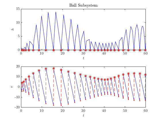
Plotting sol , we see all of the states of the composite system.

hpb = HybridPlotBuilder().subplots('on');
hpb.title('Ball Subsystem')...
    .labels('$h$', '$v$')...
    .plotFlows(sol_bb.select(1:2));
snapnow() % Show current figure in document.

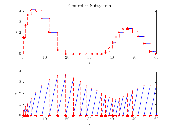
hpb.title('Controller Subsystem')...
    .labels('$u$', '$\tau$')...
    .plotFlows(sol_bb.select(3:4));
snapnow() % Show current figure in document.

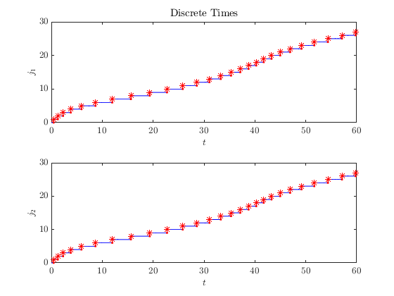
hpb.title('Discrete Times')...
    .labels('$j_1$', '$j_2$')...
    .plotFlows(sol_bb.select(5:6));

Subsystem Solutions

The solve function returns a CompositeHybridSolution object that contains all the same information as HybridSolution , but allows accessing the subsystem solutions individually (which include the state, inputs, and outputs for each subsystem). The solutions to subsystems can be accessed by placing a subsystem ID within parentheses immediately after sol .

sol_bb(1);
sol_bb(controller_subsys);
sol_bb('Ball');

Subsystem solutions have all the same properties as a HybridSolution , e.g.,

sol_bb('Ball').termination_cause

ans = 
  TerminationCause enumeration
    T_REACHED_END_OF_TSPAN

as well as the input and output values, which are stored in the properties u and y , respectively.

size(sol_bb('Ball').u)
size(sol_bb('Ball').y)

ans =
   287     1
ans =
   287     2

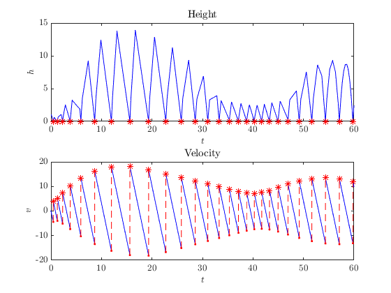
The subsystem solutions can plotted just like any other HybridSolution .

clf
hpb = HybridPlotBuilder().subplots('on')...
    .labels('$h$', '$v$')...
    .titles('Height', 'Velocity');
hpb.plotFlows(sol_bb('Ball'));

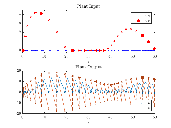
Plotting Input and Output Signals

The control signal for a subsystem can be plotted by passing the subsystem solution object and the control signal to the plotting functions in HybridPlotBuilder . If flow inputs and jump inputs are different functions, we recommend plotting flows and jumps separately. In our case, the jump input was not set, so the plot shows that the values are zero.

clf
% Plot Input Signal
subplot(2, 1, 1)
% We reuse a single HybridPlotBuilder for both plots so they are both included in the legend.
hpb = HybridPlotBuilder().title('Input Signal').jumpColor('none')...
    .filter(~sol_bb.is_jump_start)...
    .legend('$u_{C}$')...
    .plotFlows(sol_bb, sol_bb('Ball').u);
hold on
hpb.jumpMarker('*').jumpColor('r').flowColor('none')...
    .filter(sol_bb.is_jump_start)...
    .legend({'$u_D$'}, 'location', 'northeast')...
    .plotFlows(sol_bb, sol_bb('Ball').u)
title('Plant Input')
ylim('padded')

% Plot Output Signal
subplot(2, 1, 2)
HybridPlotBuilder().color('matlab')...
    .legend({'$h$', '$v$'}, 'location', 'southeast')...
    .plotFlows(sol_bb, sol_bb('Ball').y)
title('Plant Output')

Example: Single Subsystem

The CompositeHybridSystem class can also be used with a single subsystem for cases where you want to be able to modify the feedback functions without modifying the code for the system.

close() % Close figure
sys_1 = CompositeHybridSystem(ball_subsys);
sys_1.setFlowInput(1, @(y1, t, j) -5);
sys_1.setJumpInput(1, @(y1, t, j) 0);
sol_1 = sys_1.solve({x_ball_initial}, tspan, jspan);