CPS Component: Continuous-time Plant (Mobile Robot)
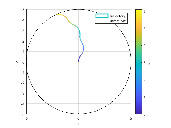
In this example a unicycle type mobile robot is simulated using the hybrid system toolbox. It is assumed that the forward velocity can be either 1 or 0, and the control command is \(u\in\mathbb{R}\) . The control input is assumed be remain between \(\pm 1\) , i.e., \(u \in [U_{\min},\ U_{\max}] := [-1,+1]\) . Moreover, the unicycle is initialized at the origin and required to reach the boundry of a circle of radius \(X_{\max}\)
Contents
The files for this example are found in the package hybrid.examples.mobile_robot :
- initialize.m
- mobile_robot.slx
- postprocess.m
The contents of this package are located in Examples\+hybrid\+examples\mobile_robot (clicking this link changes your working directory).
Mathematical Model
A unicycle mobile robot is a continuous-time nonlinear system. Let \(x_1\) and \(x_2\) be the position of the unicycle on 2D plane and \(x_3\) be the orientation. The kinematics model is given by
\[\begin{array}{ll} \dot x_1 = v \sin x_3\\ \dot x_2 = v \cos x_3\\ \dot x_3 = u, \end{array}\]
where the forward velocity \(v\) is assumed to be constant, and without loss of generality \(v = 1\) . The states and input of the system are \((x_1,x_2,x_3)\in\mathbb{R}^{3}\) and \(u \in \mathbb{R}\) , respectively. We express this system as a hybrid control system with the following data:
\[\begin{array}{ll} f(x,u):=\left[\begin{array}{c} \sin x_{3} \\ \cos x_{3} \\ u \end{array}\right], & C := \{ (x,u) \in \mathbb{R}^{3} \times \mathbb{R} \mid u \in [U_{\min},\ U_{\max}], x_1^2 + x_2^2 \leq X^2_{\max}\} \\ \\ g(x,u):=\left[ \begin{array}{c} 0 \\ 0 \\ 0 \end{array}\right], & D: = \emptyset \end{array}\]
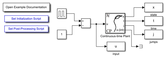
Simulink Model
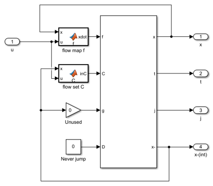
The following diagram shows the Simulink model for this example. The mobile robot is represented by the Continuous-time Plant block.
A Continuous-time Plant block contains user-defined a flow map \(f\) block and flow set \(C\) block.
The flow map and flow set functions in this example are included below.
flow map f block
function xdot = f(x, u)
    % Flow map for plant.
    xdot = [sin(x(3)); cos(x(3)); u];
end
flow set C block
function inC  = C(x, u, parameters)
    % Flow set indicator function for plant.
    x1 = x(1);
    x2 = x(2);
    minU = parameters.minU;
    maxU = parameters.maxU;
    maxX = parameters.maxX;
    if u >= minU && u <= maxU && x1^2+x2^2 <= maxX^2
        inC = 1; % report flow
    else
        inC = 0; % do not report flow
    end
end
The jump set C block is given as a constant block with value zero and the jump map D block is unused.
Example Output
The following plot shows a solution to the closed-loop system. The robot starts at the origin and then drives until it eventually hits the target set, which is a circle with radius 5 centered at the origin.