Creating and Simulating Hybrid Systems

In this tutorial, we show how to create and solve a hybrid system using the HybridSystem class. For a brief introduction to hybrid systems, see here .

Contents

• How to create a HybridSystem Subclass
• Asserting Conditions on Hybrid Systems
• Compute Solutions
• Information About Solutions
• Modifying Hybrid Arcs
• Solver Configuration Options
• Concise Hybrid System Definitions

How to create a HybridSystem Subclass

In this page, we will consider, as an example, a bouncing ball with state \(x = (x_1, x_2),\) where \(h := x_1\) is the height of the ball and \(v := x_2\) is the vertical velocity. The ball can be modeled as the following hybrid system:

\[\left\{\begin{array}{ll} \left[\begin{array}{c} \dot x_1 \\ \dot x_2 \end{array}\right] = \left[\begin{array}{c} x_2 \\ -\gamma \end{array}\right] & x \in C := \{ (x_1, x_2) \in R^2 \mid x_1 \geq 0 \textrm{ or } x_2 \geq 0 \} \\ \\ \left[\begin{array}{c} x_1^+ \\ x_2^+ \end{array}\right] = \left[\begin{array}{c} x_1 \\ -\lambda x_2 \end{array}\right] &x \in D := \{ (x_1, x_2) \in R^2 \mid x_1 \leq 0,\: x_2 \leq 0 \} \end{array} \right. \]

where \(\gamma > 0\) is the acceleration due to gravity and \(\lambda \geq 0\) is the coefficient of restitution when the ball hits the ground.

We define a MATLAB implementation of the bouncing ball in hybrid.examples.BouncingBall.m . A script for running the bouncing ball example is provided at hybrid.examples.run_bouncing_ball (the prefix hybrid.examples. indicates the package namespace that contains BouncingBall.m and run_bouncing_ball.m ). The structure of BouncingBall.m is as follows.

classdef BouncingBall < HybridSystem
    % Define bouncing ball system as a subclass of HybridSystem.
    properties
        % Define variable class properties.
        ...
    end
    properties(SetAccess = immutable)
        % Define constant (i.e., "immutable") class properties.
        ...
    end
    methods
        % Define functions, including definitions of f, g, C, and D.
        ...
    end
end

In the first line, "classdef BouncingBall < HybridSystem" specifies that BouncingBall is a subclass of the HybridSystem class, which means it inherits the attributes of that class. Within MATLAB classes, properties blocks define variables and constants that can be accessed on instances of the class. For BouncingBall , there are two properties blocks. The first defines variable variables for the system parameters \(\gamma\) and \(\lambda\) .

classdef BouncingBall < HybridSystem
    properties
        gamma = 9.8; % Acceleration due to gravity.
        lambda = 0.9; % Coefficient of bounce restitution.
    end
    ...
end

The second properties block defines constants that cannot be modified. The block attribute SetAccess = immutable means that the values cannot be changed once an object is constructed. We define two "index" constants that are useful for referencing components of the state vector x .

classdef BouncingBall < HybridSystem
    ...
    properties(SetAccess = immutable)
        % The index of 'height' component within the state vector 'x'.
        height_index = 1;
        % The index of 'velocity' component within the state vector 'x'.
        velocity_index = 2;
    end
    ...
end

For more complicated systems, it is sometimes useful to define constants for a range of indices. For example, if \(u, v \in \mathbb{R}^{4}\) and

\[x = \left[\begin{array}{c} u, v \end{array}\right],\]

then we could define the following immutable properties:

v_indices = 1:4;
u_indices = 4 + (1:4); % These parentheses are important!

Then, we can extract u and v from x as

v = x(v_indices);
u = x(u_indices);

Next, in BouncingBall , the methods block defines functions that can be called on BouncingBall objects. Every subclass of HybridSystem must define the functions flowMap , jumpMap , flowSetIndicator , and jumpSetIndicator . The indicator functions must return 1 inside their respective sets and 0 otherwise.

function xdot = flowMap(this, x, t, j)
    % Define the flow map f.
    % Set xdot to the value of f(x, t, j).
    ...
end

function xplus = jumpMap(this, x, t, j)
    % Define the jump map g.
    % Set xplus to the value of g(x, t, j).
    ...
end

function inC = flowSetIndicator(this, x, t, j)
    % Define the flow set C.
    % Set 'inC' to 1 if 'x' is in the flow set C and to 0 otherwise.
    ...
end

function inD = jumpSetIndicator(this, x, t, j)
    % Define the flow set C.
    % Set 'inD' to 1 if 'x' is in the jump set D and to 0 otherwise.
    ...
end

Notice that the first argument in each function method is this , which provides a reference to the object on which the function was called. The object's properties are referenced within the methods using this.gamma , this.lambda , etc. After the this argument, there must be one, two, or three arguments that are either (x) , (x, t) , or (x, t, j) , as needed. The full class definition of BouncingBall is shown next.

classdef BouncingBall < HybridSystem
    % A bouncing ball modeled as a HybridSystem subclass.

    % Define variable properties that can be modified.
    properties
        gamma = 9.8;  % Acceleration due to gravity.
        lambda = 0.9; % Coefficient of restitution.
    end

    % Define constant properties that cannot be modified (i.e., "immutable").
    properties(SetAccess = immutable) 
        % The index of 'height' component 
        % within the state vector 'x'. 
        height_index = 1;
        
        % The index of 'velocity' component 
        % within the state vector 'x'. 
        velocity_index = 2;
    end

    methods 
        function this = BouncingBall()
            % Constructor for instances of the BouncingBall class.

            % Call the constructor for the HybridSystem superclass and
            % pass it the state dimension. This is not strictly necessary, 
            % but it enables more error checking.
            state_dim = 2;
            this = this@HybridSystem(state_dim);
        end

        % To define the data of the system, we implement 
        % the abstract functions from HybridSystem.m

        function xdot = flowMap(this, x, t, j)
            % Extract the state components.
            v = x(this.velocity_index);

            % Define the value of f(x). 
            xdot = [v; -this.gamma];
        end

        function xplus = jumpMap(this, x)
            % Extract the state components.
            h = x(this.height_index);
            v = x(this.velocity_index);

            % Define the value of g(x). 
            xplus = [h; -this.lambda*v];
        end
        
        function inC = flowSetIndicator(this, x)
            % Extract the state components.
            h = x(this.height_index);
            v = x(this.velocity_index);

            % Set 'inC' to 1 if 'x' is in the flow set and to 0 otherwise.
            inC = (h >= 0) || (v >= 0);
        end

        function inD = jumpSetIndicator(this, x)
            % Extract the state components.
            h = x(this.height_index);
            v = x(this.velocity_index);

            % Set 'inD' to 1 if 'x' is in the jump set and to 0 otherwise.
            inD = (h <= 0) && (v <= 0);
        end
    end
end

An instance of the BouncingBall class is then created as follows:

bb_system = hybrid.examples.BouncingBall();

Values of the properties can be modified using dot indexing on the object:

bb_system.gamma = 3.72;
bb_system.lambda = 0.8;

For more information about writing MATLAB classes, see the online MATLAB documentation .

WARNING: The functions flowMap , flowSetIndicator , and jumpSetIndicator must be deterministic—each time they are called for a given set of inputs (x, t, j) , they must return the same output values. In other words, flowMap , flowSetIndicator , and jumpSetIndicator must be functions in the mathematical sense. If they depend on system parameters stored as object properties, then those parameters must be constant during each execution of HybridSystem.solve (described below). It is okay to change the system parameters in between calls to solve , but all values that change during a solution, must be included in the state vector x .

The reason for this warning is that modifying system parameters within flowMap , flowSetIndicator , or jumpSetIndicator will produce unpredictable behavior because the hybrid solver does not move monotonically forward in time; Sometimes, the solver backtracks while computing a solution to \(\dot{x} = f(x),\) such as when searching for the time when \(x\) enters \(D\) or leaves \(C\) . The jumpMap , on the other hand, can be nondeterministic, such as including random noise, without causing the same sort of problems because the solver never backtracks across a jump.

To protect against accidentally modifying system parameters, each parameter can be stored as an immutable object property that is set when the HybridSystem object is constructed. The value of an immutable property cannot be modified after an object is created. An example of how to implement an immutable property is included here:

classdef MyHybridSystem < HybridSystem
   properties(SetAccess=immutable)
       my_property % cannot be modified except in the constructor
   end
   methods
       function this = MyHybridSystem(my_property) % Constructor
           this.my_property = my_property; % set immutable property value.
       end
   end
end

The value of my_property is set when a MyHybridSystem is constructed:

sys = MyHybridSystem(3.14);
assert(sys.my_property == 3.14)

For more information about immutable properties see the MATLAB documentation here .

Asserting Conditions on Hybrid Systems

When implementing a hybrid system, it is helpful to verify that certain points are or are not in \(C\) or in \(D.\) This is accomplished in HybridSystem with four functions: assertInC , assertInD , assertNotInC , and assertNotInD .

% Define some points.
x_ball_above_ground = [1; 0];
x_ball_at_ground    = [0; 0]; % and stationary
x_ball_below_ground = [-1; -1]; % and moving down

% Check the above-ground point.
bb_system.assertInC(x_ball_above_ground);
bb_system.assertNotInD(x_ball_above_ground);

% Check the at-ground point.
bb_system.assertInC(x_ball_at_ground);
bb_system.assertInD(x_ball_at_ground);

% Check the below-ground point.
bb_system.assertNotInC(x_ball_below_ground);
bb_system.assertInD(x_ball_below_ground);

In addition to checking that a given point is in the desired set, the functions assertInC , assertInD check that the flow or jump map, respectively, can be evaluated at the point and produces a vector with the correct dimensions.

If an assertion fails, as in following code, then an error is thrown and execution is terminated (unless caught by a try-catch block):

try
    bb_system.assertInD(x_ball_above_ground) % This fails.
catch e
    fprintf(2,'Error: %s\n', e.message);
end

Error: The point
  x: [1;0]
was expected to be inside D but was not.

Compute Solutions

A numerical approximation of a solution to the hybrid system is computed by calling the solve function. The solve function returns a HybridSolution object that contains information about the (approximate) solution (use the properties t , j , and x to recover the standard output from HyEQSolver ). To compute a solution, pass the initial state and time spans to the solve function ( solve is defined in the HybridSystem class and bb_system is a HybridSystem object because BouncingBall is a subclass of HybridSystem ). Optionally, a HybridSolverConfig object can be passed to the solver to set various configurations (see below).

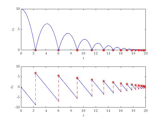
x0 = [10, 0];
tspan = [0, 20];
jspan = [0, 30];
config = HybridSolverConfig('refine', 32); % Improves plot smoothness for demo.
sol = bb_system.solve(x0, tspan, jspan, config);
plotFlows(sol); % Display solution

The use of HybridSolverConfig is described below, in "Solver Configuration Options"

The option 'refine' for HybridSolverConfig causes computed ODE solutions to be smoothly interpolated between timesteps. For documentation about plotting hybrid arcs, see Plotting Hybrid Arcs .

Information About Solutions

The return value of the solve method is a HybridSolution object that contains information about the solution.

sol

sol = 
  HybridSolution with properties:

                      x0: [2×1 double]
                      xf: [2×1 double]
       termination_cause: T_REACHED_END_OF_TSPAN
                       t: [4111×1 double]
                       j: [4111×1 double]
                       x: [4111×2 double]
            flow_lengths: [15×1 double]
              jump_times: [14×1 double]
    shortest_flow_length: 0.1515
       total_flow_length: 20
              jump_count: 14

A description of each HybridSolution property is as follows:

• t : The continuous time values of the solution's hybrid time domain.
• j : The discrete time values of the solution's hybrid time domain.
• x : The state vector of the solution.
• x0 : The initial state of the solution.
• xf : The final state of the solution.
• flow_lengths : the durations of each interval of flow.
• jump_times : the continuous times when each jump occured.
• shortest_flow_length : the length of the shortest interval of flow.
• total_flow_length : the length of the entire solution in continuous time.
• jump_count : the number of discrete jumps.
• termination_cause : the reason that the solution terminated.

The possible values for termination_cause are

• STATE_IS_INFINITE
• STATE_IS_NAN
• STATE_NOT_IN_C_UNION_D
• T_REACHED_END_OF_TSPAN
• J_REACHED_END_OF_JSPAN
• CANCELED

Modifying Hybrid Arcs

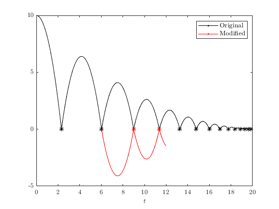
Often, after calculating a solution to a hybrid system, we wish to manipulate the resulting data, such as evaluating a function along the solution, removing some of the components, or truncating the hybrid domain. Several functions to this end are included in the HybridArc class ( HybridSolution is a subclass of HybridArc , so the solutions generated by HybridSystem.solve are HybridArc objects). In particular, the functions are select , transform , restrictT and restrictJ . See doc('HybridArc') for details.

hybrid_arc = sol.select(1);                   % Pick the 1st component.
hybrid_arc = hybrid_arc.transform(@(x) -x);   % Negate the value.
hybrid_arc = hybrid_arc.restrictT([1.5, 12]); % Truncate to t-values between 4.5 and 7.
hybrid_arc = hybrid_arc.restrictJ([2, inf]);  % Truncate to j-values >= 2.

% Plot hybrid arcs
clf
hpb = HybridPlotBuilder();
hpb.color('black').legend('Original').plotFlows(sol.select(1));
hold on
hpb.color('red').legend('Modified').plotFlows(hybrid_arc)

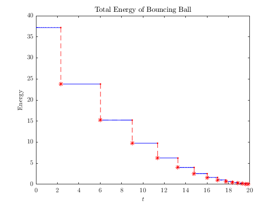
Example: Suppose we want to compute the total energy of the bouncing ball:

\[E(x) = \gamma x_1 + \frac{1}{2} x_2^2.\]

We can map the HybridArc object sol to a new HybridArc with the transform function. (Note that the state dimension before ( \(n=2\) ) and after ( \(n=1\) ) are not the same.)

clf
energy_fnc = @(x) bb_system.gamma*x(1) + 0.5*x(2)^2;
plotFlows(sol.transform(energy_fnc))
title('Total Energy of Bouncing Ball')
ylabel('Energy')

You can also construct a HybridArc directly from the values of t , j , and x as follows:

t = linspace(0, 10, 100)'; % Must be a column vector
j = zeros(100, 1);
x = t.^2;
hybrid_arc = HybridArc(t, j, x)

hybrid_arc = 
  HybridArc with properties:

                       t: [100×1 double]
                       j: [100×1 double]
                       x: [100×1 double]
            flow_lengths: 10
              jump_times: [0×1 double]
    shortest_flow_length: 10
       total_flow_length: 10
              jump_count: 0

Solver Configuration Options

To configure the hybrid solver, create a HybridSolverConfig object and pass it to solve as follows:

config = HybridSolverConfig('AbsTol', 1e-3);
bb_system.solve(x0, tspan, jspan, config);

There are three categories of options that can be configured with HybridSolverConfig :

1. Jump/Flow Priority for determining the behavior of solutions in \(C \cap D\) .
2. ODE solver options.
3. Hybrid solver progress updates options.

Jump/Flow Priority

By default, the hybrid solver gives precedence to jumps when the solution is in the intersection of the flow and jump sets. This can be changed by setting the priority to one of the (case insensitive) strings 'flow' or 'jump' . For an example for how changing the priority affects solutions, see Behavior in the Intersection of C and D (the linked example uses Simulink instead of MATLAB, which has an additional "random" priority mode, not currently supported in the MATLAB HyEQ library).

config.priority('flow');
config.priority('jump');

ODE Solver Options

The ODE solver function and solver options can be modified in config . To set the ODE solver, pass the name of the ODE solver function name to the odeSolver function. The default is 'ode45' . For guidence in picking an ODE solver, see this list .

config.odeSolver('ode23s');

Most of the options for the builtin MATLAB ODE solvers (described here ) can be set within HybridSolverConfig . A list of supported functions is provided below. To set an ODE solver option, use the odeOption function:

config.odeOption('AbsTol', 1e-3); % Set the absolute error tolerance for each time step.

Several commonly used options can be set by passing name-value pairs to the HybridSolverConfig constructor. The options that can be set this way are 'odeSolver' , 'RelTol' , 'AbsTol' , 'MaxStep' , 'Jacobian' , and 'Refine' .

config = HybridSolverConfig('odeSolver', 'ode23s', ...
                            'RelTol', 1e-3, 'AbsTol', 1e-4,  ...
                            'MaxStep', 0.5, 'Refine', 4);

% Display the options struct.
config.ode_options

ans = 
  struct with fields:

              AbsTol: 1.0000e-04
                 BDF: []
              Events: []
         InitialStep: []
            Jacobian: []
           JConstant: []
            JPattern: []
                Mass: []
        MassSingular: []
            MaxOrder: []
             MaxStep: 0.5000
         NonNegative: []
         NormControl: []
           OutputFcn: []
           OutputSel: []
              Refine: 4
              RelTol: 1.0000e-03
               Stats: []
          Vectorized: []
    MStateDependence: []
           MvPattern: []
        InitialSlope: []

Some of the ODE solver options have not been tested with the hybrid equation solver. The following table lists all ODE solver options and information about whether the HyEQ solver supports each. For a description of each option, see doc('odeset').

ODE Option	Supported?
RelTol	Yes
AbsTol	Yes
NormControl	Untested
NonNegative	Untested
OutputFcn	No. Use 'progress' function.
OutputSel	Untested
Refine	Yes
Stats	Yes, but will print stats after each interval of flow.
InitialStep	Untested
MaxStep	Yes
Events	No
Jacobian	Yes
JPattern	Yes
Vectorized	Untested, but probably won't work.
Mass	Untested
MStateDependence	Untested
MvPattern	Untested
MassSingular	Untested
InitialSlope	Yes, for DAEs

Progress Updates

Computing a hybrid solution can take considerable time, so progress updates are displayed. Progress updates can be disabled by passing 'silent' to config.progess() .

config.progress('silent');

% To restore the default behavior:
config.progress('popup');

For brevity, 'silent' can be also be passed as the first argument to the HybridSolverConfig constructor.

HybridSolverConfig('silent', );

Alternatively, 'silent' can be passed directly to solve in place of config , if no other solver configurations are desired.

bb_system.solve(x0, tspan, jspan, 'silent');

Concise Hybrid System Definitions

We also provide a quicker way to create a hybrid system in-line instead of creating a new subclass of HybridSystem. This approach creates systems that are slower to solve and harder to debug, so use with care—creating a subclass of HybridSystem is the recommended method for defining complicated systems.

system_inline = HybridSystemBuilder() ...
            .f(@(x, t) t*x) ...
            .g(@(x) -x/2) ...
            .C(@(x) 1) ...
            .D(@(x, t, j) abs(x) >= j) ...
            .build();
sol_inline = system_inline.solve(0.5, [0, 10], [0, 10]);

The functions f , g , C and D can have 1, 2, or 3 input arguments, namely (x) , (x,t) , or (x, t, j) .

The definition of hybrid systems can be made even more concise by passing function handles for f , g , C and D to the HybridSystem function, which constructs a HybridSystem with the given data. Again, this approach is slower and harder to debug, so it is not generally recommended.

f = @(x, t) t*x;
g = @(x) -x/2;
C = @(x) 1;
D = @(x, t, j) abs(x) >= j;
system_inline = HybridSystem(f, g, C, D);