CPS Component: Analog-to-Digital Converter (ADC)
In this example, an analog-to-digital converter (ADC) is modeled in Simulink as a hybrid system with an input, where the input is sampled periodically by the ADC.
Contents
The files for this example are found in the package hybrid.examples.analog_to_digital_converter :
- initialize.m
- adc.slx
- postprocess.m
and in the package hybrid.examples.bouncing_ball_with_adc :
- initialize.m
- ball_with_adc.slx
- postprocess.m
The contents of these packages are located in Examples\+hybrid\+examples\bouncing_ball_with_adc and Examples\+hybrid\+examples\analog_to_digital_converter (clicking these links changes your working directory).
Mathematical Model
The ADC is modeled as a hybrid system with the following data:
\[\begin{array}{ll} f(x,u):=\left[\begin{array}{c} 0 \\ 1 \end{array}\right], & C := \{ (x,u) \in \mathbb{R}^2 \times \mathbb{R} \mid (x_2 \geq 0) \wedge (x_2 \leq T_s) \} \\ \\ g(x,u):=\left[ \begin{array}{c} u \\ 0 \end{array}\right], & D: = \{(x,u) \in \mathbb{R}^2 \times \mathbb{R} \mid x_2 > T_s \} \end{array}\]
where \(u\) is the input to the ADC, \(x_1\) is a memory state used to store the samples of \(u\) , \(x_2\) is a timer that causes the ADC to sample \(u\) every \(T_s\) seconds, and \(T_s > 0\) denotes the time between samples of \(u\) .
Steps to Run Model
The following procedure is used to simulate this example:
- Open hybrid.examples.analog_to_digital_converter.adc.slx .
- Double-click the block labeled Double Click to Initialize .
- To start the simulation, click the run button or select Simulation>Run .
- Once the simulation finishes, click the block labeled Double Click to Plot Solutions . Several plots of the computed solution will open.
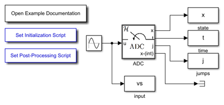
Simulink Model
The following diagram shows the Simulink model of the bouncing ball. The contents of the blocks flow map f , flow set C , etc., are shown below. When the Simulink model is open, the blocks can be viewed and modified by double clicking on them.
The following Matlab embedded functions that describe the sets \(C\) and \(D\) and the functions \(f\) and \(g\) for the ADC system.
flow map f block
function xdot = f(x, u)
    % Flow map for analog to digial converter.
    msdot = 0*u;       % measured continuous dynamics
    tau_dot = 1;       % Timer tau_s
    xdot = [msdot; tau_dot];
end
flow set C block
function inC  = C(x, u, sample_time)
    % Flow set indicator function for analog to digial converter.
    tau = x(end); % timer state
    if tau >= 0 && tau <= sample_time
        inC = 1;      % report flow
    elseif tau> sample_time
        inC = 0;      % do not report flow
    else
        inC = 0;
    end
end
jump map g block
function xplus = g(x, u)
    % Jump map for for analog to digial converter.
    msplus = u;        % output = measured input
    tau_plus = 0;     % Timer tau_s
    xplus = [msplus; tau_plus];
end
jump set D block
function inD  = D(x, u, sample_time)
    % Jump set indicator function for analog to digial converter.
    tau = x(end); % timer state
    if tau >= 0 && tau <= sample_time
        inD = 0;          % do not report jump
    elseif tau > sample_time
        inD = 1;          % report jump
    else
        inD = 0;
    end
end
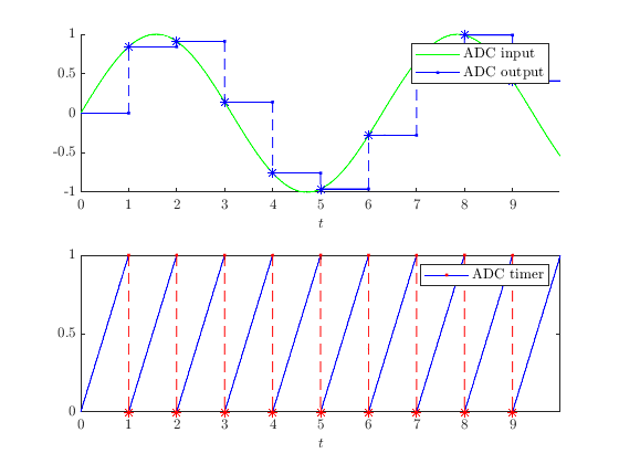
Example Output
Let the input function be \(u(t,j) = \sin(t)\) and let \(T_s = \pi/8\) . The solution to the ADC system from \(x(0,0)=[0,0]^\top\) and with T=10 , J=20, |rule=1 shows that the ADC samples the sinusoidal input every \(\pi/8\) seconds.
ADC Connected to Bouncing Ball
In this section, the interconnection of a bouncing ball system and an ADC is modeled in Simulink. This shows how an ADC block can be used to discretize a hybrid system.
The model of the ADC is the same as above and the model of the bouncing ball subsystem is described in Modeling a Hybrid System with Embedded Function Blocks (Bouncing Ball with Input) .
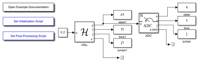
Simulink Model for ADC Connected to Bouncing Ball
The following diagram shows the Simulink model with an ADC subsystem connected to the output of a bouncing ball subsystem. (The ball subsystem is given here .)
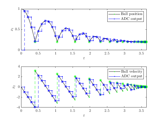
Example Output
Let the input function to the bouncing ball be \(u(t,j) = 0.2\) and let \(\gamma = -9.81\) , \(\lambda = 0.8\) , and \(T_s = 0.1\) . The solution to the interconnection from an initial condition of \(x(0,0)=[0,0]^\top\) for the bouncing ball and \(x(0,0)=[0,0]^\top\) for the ADC, and with T=10, J=20, rule=1 , shows that the ADC samples the ball position and velocity every \(0.1\) seconds.