Composing Multiple Hybrid Subsystems (Bouncing Ball on Moving Platform)
In this example, a ball bouncing on a moving platform is modeled in Simulink as a pair of interconnected hybrid systems with inputs.
Contents
The files for this example are found in the package hybrid.examples.coupled_subsystems :
- initialize.m
- coupled.slx
- postprocess.m
The contents of this package are located in Examples\+hybrid\+examples\coupled_subsystems (clicking this link changes your working directory).
Mathematical Model
Consider a bouncing ball \(\mathcal{H}_1\) bouncing on a moving platform \(\mathcal{H}_2\) . The ball accelerates due to gravity and both the ball and platform have discrete changes in velocity due to collisions between them. This problem lends itself to being modeled by a pair of interconnected hybrid systems because the states of each system affect the behavior of the other system. In this interconnection, the bouncing ball will contact the platform, bounce back up, and pushing the platform toward the ground. In order to model this system, the output of the bouncing ball becomes the input of the moving platform, and vice versa. The model includes disturbances to the velocities of the ball and platform.
The bouncing ball is modeled as a hybrid subsystem \(\mathcal{H}_1\) with
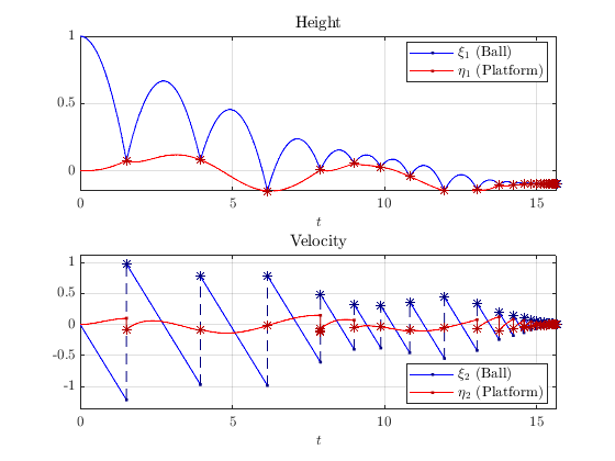
- state \(\xi = [\xi_1 ,\xi_2]^\top\) where \(\xi_1\) is the height of the ball and \(\xi_2\) is its velocity,
- output \(y_1 \in \mathbb{R}\) , which is set to the height of the ball,
- inputs \(u_1 \in \mathbb{R}\) , which is set to the height of the platform, and
- disturbances \(v_1 = [v_{11} , v_{12}]^\top \in \mathbb{R}^{2}\) to the velocity of the ball during flows and jumps, respectively.
The model of \(\mathcal{H}_1\) is then given as
\[\left\{\begin{array}{ll} f_1(\xi, u_1,v_1):=\left[\begin{array}{c} \xi_2 \\ -\gamma + v_{11} \end{array}\right], & C_1 : = \{(\xi,u_1) \mid \xi_1 \geq u_1, u_1 \geq 0\} \\ \\ g_1(\xi, u_1, v_1):=\left[\begin{array}{c} \xi_1 \\ \lambda|\xi_2| + v_{12} \end{array}\right], &D_1: =\{(\xi,u_1) \mid \xi_1 =u_1, u_1 \geq 0\}, \\ \\ y_1 = h_1(\xi) := \xi_1 \end{array}\right. \]
where \(\gamma>0\) is the acceleration due to gravity, and \(\lambda \in [0,1)\) is the cofficient of restitution for collisions between the ball and the platform.
The platform is modeled as a hybrid subsystem \(\mathcal{H}_2\) with
- state \(\eta = [\eta_1 , \eta_2]^\top \in \mathbb{R}^{2}\) where \(\eta_1\) is the height of the platform and \(\eta_2\) is its velocity,
- output \(y_2 \in \mathbb{R}\) is set to the height of the platform,
- intput \(u_2 \in \mathbb{R}\) is set to the height of the ball, and
- disturbances \(v_2 = [v_{21} , v_{22}]^\top \in \mathbb{R}^{2}\) to velocity of the platform during flows and jumps, respecitvely.
The model of the platform system \(\mathcal{H}_2\) is given by
\[\left\{\begin{array}{ll} f_2(\eta,u_2,v_2):=\left[\begin{array}{c} \eta_2 \\ -\eta_1-\beta\eta_2 +v_{12} \end{array} \right], & C_2 : = \{(\eta,u_2) \mid \eta_1 \leq u_2, \eta_1 \geq 0\} \\ \\ g_2(\eta,u_2,v_2):=\left[\begin{array}{c} \eta_1 \\ -\lambda|\eta_2| + v_{22} \end{array} \right], & D_2: =\{(\eta,u_2) \mid \eta_1 = u_2, \eta_1 \geq 0 \}, \\ \\ y_2 = h_2(\eta) := \eta_1, \end{array}\right.\]
where \(\beta \geq 0\) is a velocity damping coefficient.
The interconnection between \(\mathcal H_1\) and \(\mathcal H_2\) is defined by the input assignment
\[u_1 = y_2, \quad u_2 = y_1.\]
The signals \(v_1\) and \(v_2\) are included as external inputs to the model to simulate the effects of environmental perturbations, such as a wind gust, on the system.
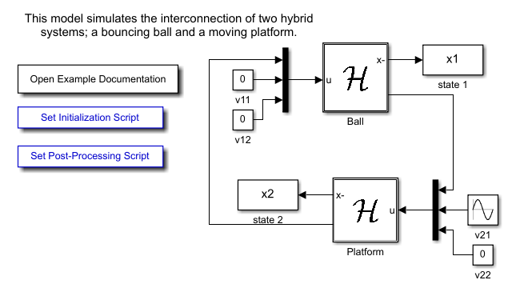
Simulink Model
The following diagram shows the Simulink model for the interconnected hybrid systems. The contents of the blocks flow map f , flow set C , etc., are shown below.
The Simulink blocks for the bouncing ball \(\mathcal{H}_{1}\) :
flow map f block
function xi_dot = f1(xi, u)
    % Flow map for ball in Example 1.6

    % Magnitude of acceleration due to gravity.
    gravity = 0.8;

    % Input from disturbances.
    v11 = u(2);
    v12 = u(3);

    % Flow map
    xi1_dot = xi(2);
    xi2_dot = -gravity + v11;

    xi_dot = [xi1_dot; xi2_dot];
end
flow set C block
function inC  = C1(xi, u)
    % Flow set indicator for ball in Example 1.6

    % Input from platform's output.
    y21 = u(1); % Height of platform.

    if (xi(1) >= y21 || xi(2) >= 0)
        inC = 1; % report flow
    else
        inC = 0; % do not report flow
    end
end
jump map g block
function xi_plus = g1(xi, u)
    % Jump map for ball in Example 1.6

    % Constants
    lambda = 0.8; % Coefficient of restitution.

    % Input from disturbances.
    v11 = u(2);
    v12 = u(3);

    xi_plus = [xi(1); lambda*abs(xi(2)) + v12];
end
jump set D block
function inD = D1(xi, u)
    % Jump set indicator function for ball in Example 1.6

    % Input from platform's output.
    y21 = u(1); % Height of platform.

    if (xi(1) <= y21 && xi(2) <= 0)
        inD = 1; % report jump
    else
        inD = 0; % do not report jump
    end
end
The Simulink blocks for the moving platform \(\mathcal{H}_{2}\) :
flow map f block
function eta_dot = f2(eta, u)
% Flow map for platform in Example 1.6.

    % Constants
    beta = 2; % Velocity damping coefficient.

    % Input from disturbances.
    v21 = u(2);
    v22 = u(3);

    % flow map
    eta1_dot = eta(2);
    eta2_dot = -eta(1)-beta*eta(2)+v21;

    eta_dot = [eta1_dot; eta2_dot];
end
flow set C block
function inC  = C2(eta, u)
    % Flow set indicator function for platform in Example 1.6.

    % Input from balls's output.
    y1 = u(1); % Height of ball.

    if (eta(1) <= y1)
        inC = 1;  % report flow
    else
        inC = 0;  % do not report flow
    end
end
jump map g block
function eta_plus = g2(eta, u)
% Jump map for platform in Example 1.6.

    % Constants
    lambda  = 0.8; % Coefficient of bounce restitution.

    % Input from disturbances.
    v21 = u(2);
    v22 = u(3);

    % Jump map
    eta_plus = [eta(1); -lambda*abs(eta(2))+v22];
end
jump set D block
function inD  = D2(eta, u)
    % Jump set indicator function for platform in Example 1.6.

    % Input from balls's output.
    y1 = u(1); % Height of ball.

    if (eta(1) >= y1)
        inD = 1; % Report jump
    else
        inD = 0; % Do not report jump
    end
end
Example Output
A solution to the composition of \(\mathcal{H}_1\) and \(\mathcal{H}_2\) is shown below with \(\gamma = 0.8\) , \(\beta=2\) , T=18 , J=20 , and rule=1 . The inputs \(v_{11}\) , \(v_{12}\) , \(v_{22}\) are zero and \(v_{21}\) is a sinusoidal signal.