CPS Component: Finite State Machine
In this example, a finite state machine (FSM) is modeled in Simulink as a hybrid system with an input, where the input triggers the discrete transitions (or jumps).
Contents
The files for this example are found in the package hybrid.examples.finite_state_machine :
- initialize.m
- fsm.slx
- postprocess.m
The contents of this package are located in Examples\+hybrid\+examples\finite_state_machine (clicking this link changes your working directory).
Mathematical Model
A finite state machine (FSM), also called a deterministic finite automaton (DFA) is a system with inputs, states, and outputs taking values from finite sets that are updated at discrete transitions (or jumps) triggered by its inputs. For a FSM with state \(q \in Q\) and input \(u \in \Sigma,\) the update mechanism at jumps is determined by the difference equation
\[q^+ = \delta(q,u) \qquad (q,u) \in Q \times \Sigma \]
and the output of the system is
\[y = h(q) \qquad q \in Q.\]
The FSM system is modeled as a hybrid system with the following data:
\[\begin{array}{ll} f(q,u):=\left[\begin{array}{c} 0 \\ 0 \end{array}\right], & C := \{ (q,u) \in Q \times \Sigma \mid \delta(q, u) = q \} \\ g(q,u):= \delta(q, u) = \left[ \begin{array}{c} u_{1} + u_2 \\ u_1 - u_{2} \end{array}\right], & D: = \{ (q,u) \in Q \times \Sigma \mid \delta(q, u) \neq q\} \\ y:= h(q) = q \end{array}\]
where the state is given by \(q = (q_{1}, q_{2})\in Q := \{0, 1, 2\}\times \{-1, 0, 1\}\) and the input is given by \(u = (u_{1}, u_{2})\in \Sigma := \{0, 1\}\times \{0, 1\}\) .
Steps to Run Model
The following procedure is used to simulate this example using the model in the file FSM_example.slx :
- Open hybrid.examples.finite_state_machine.fsm.slx in Simulink (clicking this link changes your working directory and opens the model).
- Double-click the block labeled Double Click to Initialize .
- To start the simulation, click the run button or select Simulation>Run .
- Once the simulation finishes, click the block labeled Double Click to Plot Solutions . Several plots of the computed solution will open.
Simulink Model
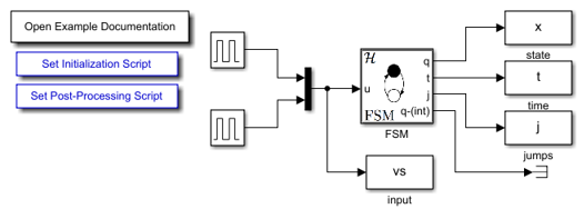
The following diagram shows the Simulink model of the FSM. When the Simulink model is open, the blocks can be viewed and modified by double clicking on them.

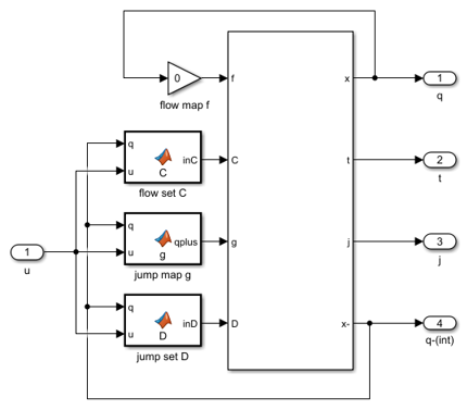
The interior of the FSM block is shown here.

The functions used to define \(g, C,\) and \(D\) in the FSM blocks are included below. When using the finite state machine block, these functions should be modified to in accordance with the system being modeled.
flow set C block
function inC  = C(q, u)
    % Flow set indicator function for finite state machine.
    qplus = zeros(size(q)); % dynamics of the q state, e.g.,     qplus(1) = u(1)+u(2);
    qplus(1) = u(1) + u(2);
    qplus(2) = u(1) - u(2);
    if q(1)==qplus(1) && q(2)==qplus(2)
        inC = 1; % report flow
    else
        inC = 0; % do not report flow
    end
end
jump map g block
function qplus = g(q, u)
    % Jump map for finite state machine.
    qplus = zeros(size(q));
    qplus(1) = u(1) + u(2);
    qplus(2) = u(1) - u(2);
end
jump set D block
function inD  = D(q, u)
    % Jump set indicator for finite state machine.

    qplus = zeros(size(q)); % dynamics of the q state e.g.,
    qplus(1) = u(1) + u(2);
    qplus(2) = u(1) - u(2);
    if q(1)==qplus(1) && q(2)==qplus(2)
        inD = 0; % do not report jump
    else
        inD = 1; % report jump
    end
end
Example Output
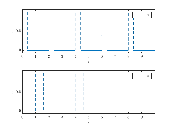
Let the input function be
\[\begin{array}{ll} u_{1}(t,u):=\left\{\begin{array}{ll} 1 & \textrm{if } t\in[2k,\ 2k + 0.4) = [0, 0.4) \cup [2, 2.4) \cup \cdots \\ 0 & \textrm{otherwise} \\ \end{array}\right., \\ \\ u_{2}(t,u):=\left\{\begin{array}{ll} 1 & \textrm{if } t\in[3k + 1,\ 3k + 1.6) = [1, 1.6) \cup [4, 4.6) \cup \cdots\\ 0 & \textrm{otherwise} \\ \end{array}\right. \end{array} \]
for all \(k\in \mathbb{N}\) .

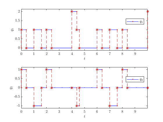
The solution to the FSM system from \(x(0,0)=[0,0]^\top\) and with T=10 , J=20 , rule=1 shows the mode transition of the FSM system. By comparing with the prior figure, we see that \(q_1 = u_1 + u_2\) and \(q_2 = u_1 - u_1,\) as expected.
