Example Hybrid System with External Functions (Bouncing Ball)
In this example, a bouncing ball is modeled in Simulink as a hybrid system.
Contents
The files for this example are found in the package hybrid.examples.bouncing_ball :
- initialize.m
- bouncing_ball.slx
- C.m , f.m , D.m , g.m
- postprocess.m
The contents of this package are located in Examples\+hybrid\+examples\bouncing_ball (clicking this link changes your working directory).
For the same system modeled using the MATLAB-based HyEQ solver, see here .
Mathematical Model
The bouncing ball is modeled as a hybrid system with the following data:
\[\begin{array}{ll} f(x) := \left[\begin{array}{c} x_{2} \\ -\gamma \end{array}\right], & C := \{ x \in \mathbb{R}^{2} \mid x_{1} \geq 0 \} \\ \\ g(x) := \left[ \begin{array}{c} 0 \\ -\lambda x_{2} \end{array}\right], & D := \{x \in \mathbb{R}^2 \mid x_1 \leq 0,\ x_2 \leq 0\} \end{array}\]
where \(\gamma > 0\) is the acceleration due to gravity and \(\lambda \in [0,1)\) is the coefficient of restitution. For this example, we consider a ball bouncing on a floor at zero height.
Simulink Model
The following diagram shows the Simulink model of the bouncing ball. When the Simulink model is open, the blocks can be viewed and modified by double clicking on them.

Double-click black hybrid system \(\mathcal{H}\) block open a dialog box where you can specify function handles for \(f\) , \(g\) , \(C\) , and \(D\) , and other system configuration options.
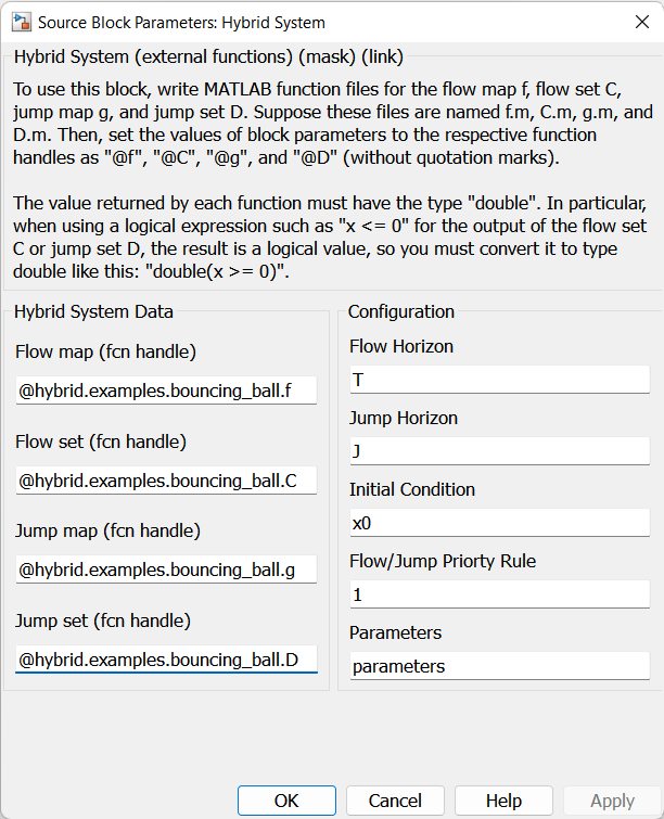
To "look inside" the block, click the arrow in the lower-left corner of the block or open the block's context menu and select Mask > Look Under Mask. (To implement a hybrid system with external functions, you do not need to modify anything under the mask. All the necessary configuration is done in the mask dialog box.) The contents of the hybrid system block are shown here.
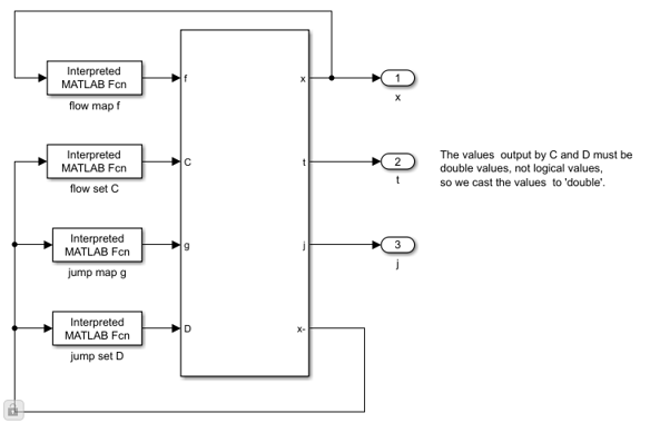
The flow map f , flow set C , jump map g , and jump set D are defined by interpreted MATLAB function blocks. These blocks call the MATLAB functions chosen in the mask dialog, namely C.m , f.m , D.m , g.m in the hybrid.examples.bouncing_ball package. The MATLAB source code each function is included below.
f.m:
function xdot = f(x, parameters)
    % Flow map for Bouncing Ball.
    gamma = parameters.gamma; % Acceleration due to gravity.
    xdot = [x(2); gamma];
end
C.m:
function inside_C = C(x, ~)
    % Flow set for Bouncing Ball.
    % Return 0 if outside of C, and 1 if inside C
    if x(1) >= 0 % Flow if height is nonnegative.
        inside_C = 1;
    else
        inside_C = 0;
    end
end
g.m:
function xplus = g(x, parameters)
    % Jump map for Bouncing Ball.
    lambda = parameters.lambda; % Coefficient of bounce restitution.
    xplus = [-x(1); -lambda*x(2)];
end
D.m:
function inside_D = D(x, ~)
    % Jump set for Bouncing Ball.
    % Return 0 if outside of D, and 1 if inside D
    if (x(1) <= 0 && x(2) <= 0)
        inside_D = 1;
    else
        inside_D = 0;
    end
end
How to Run
The following procedure is used to simulate this example:
- Open hybrid.examples.bouncing_ball.bouncing_ball . It may take a few seconds for Simulink to open.
- In Simulink, double click the block "Double Click to Initialize" to initialize values (initial conditions, parameters, etc.).
- Start the simulation by clicking the "Run" button. Let the simulation finish.
- Double click the block "Double Click to Plot Solutions" to generate plots .
Solution
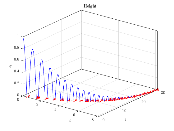
A solution to the bouncing ball system from \(x(0,0)=[1,0]^\top\) and with TSPAN = [0 10] , JSPAN = [0 20] , rule = 1 , \(g = -9.8\) , and \(\lambda = 0.9\) is shown plotted against continuous time \(t\) :

and against discrete time \(j\) :
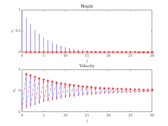
The next plot depicts the corresponding hybrid arc for the position state.