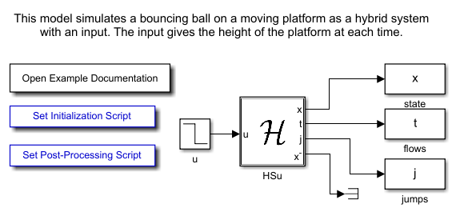
Example Hybrid System with Embedded Functions (Bouncing Ball with Input)
In this example, a ball bouncing on a moving platform is modeled in Simulink as a hybrid system with an input, where the input determines the height of the platform.
Contents
The files for this example are found in the package hybrid.examples.bouncing_ball_with_input :
- initialize.m
- ball_with_input.slx
- ball_with_input2.slx
- postprocess.m
The contents of this package are located in Examples\+hybrid\+examples\bouncing_ball_with_input (clicking this link changes your working directory).
Mathematical Model
The bouncing ball system on a moving platform is modeled as a hybrid system with the following data:
\[\left\{\begin{array}{ll} f(x,u):=\left[\begin{array}{c} x_{2} \\ -\gamma \end{array}\right], & C := \{ (x,u) \in \mathbb{R}^{2} \times \mathbb{R} \mid x_{1} \geq u \} \\ \\ g(x,u):=\left[ \begin{array}{c} u \\ -\lambda x_{2} \end{array}\right], & D: = \{ (x,u) \in \mathbb{R}^{2} \times \mathbb{R} \mid x_{1} \leq u, \ x_{2} \leq 0\} \end{array}\right.\]
where \(\gamma >0\) is the acceleration due to gravity, \(u\) is the height of the platform given as an input, and \(\lambda \in [0,1)\) is the coefficient of restitution.
Steps to Run Model
The following procedure is used to simulate this example using the model in the file Example_1_3.slx :
- Open hybrid.examples.bouncing_ball_with_input.ball_with_input.slx in Simulink.
- In Simulink, double click the block "Double Click to Initialize" to initialize variables (parameters, initial values, etc.).
- Start the simulation by clicking the "Run" button. Let the simulation finish.
- Double click the block "Double Click to Plot Solutions" to generate plots
Simulink Model
The following diagram shows the Simulink model of the bouncing ball. When the Simulink model is open, the blocks can be viewed and modified by double clicking on them.
Looking inside the hybrid system block 'HS' shows that the functions \(f, g, C,\) and \(D\) are defined using MATLAB function blocks The contents of the blocks flow map f , flow set C , etc., are shown below.
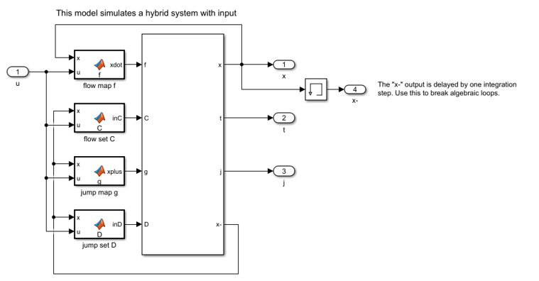
The Simulink blocks for the hybrid system in this example are included below. The Embedded MATLAB function blocks f, C, g, D are edited by double-clicking on the blocks in Simulink.
flow map f block
function xdot = f(x, u, parameters)
    % Flow map for Bouncing Ball with Input
    v = x(2);
    xdot = [v; parameters.gamma];
end
flow set C block
function inC  = C(x, u)
    % Flow set indicator for Bouncing Ball with Input
    h = x(1);
    if (h >= u)  % flow condition
        inC = 1; % report flow
    else
        inC = 0; % do not report flow
    end
end
jump map g block
 function xplus = g(x, u, parameters)
    % Jump map for Bouncing Ball with Input
    lambda = parameters.lambda;
    v = x(2);
    xplus = [u; -lambda*v];
end
jump set D block
function inD  = D(x, u)
    % Jump set indicator function for Bouncing Ball with Input.
    h = x(1);
    v = x(2);
    if (h <= u) && (v <= 0) % jump condition
        inD = 1; % report jump
    else
        inD = 0; % do not report jump
    end
end
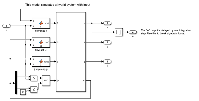
Alternative Simulink Model
Above, the functions \(f, g, C,\) and \(D\) are defined using MATLAB function blocks, but in some cases, one may want to use other Simulink blocks instead of writing custom functions. The Simulink model, below, shows the jump set D modeled in Simulink using operational blocks instead of a MATLAB function block.
Example Output
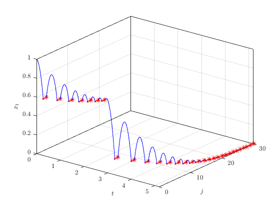
Let the input function be \(u(t,j) = 0.6\) for \(t \in [0, 2.5)\) and \(u(t, j) = 0\) for \(t \geq 2\) , and let \(\gamma = 9.81\) and \(\lambda=0.8\) . The solution to the bouncing ball system from \(x(0,0)=[1,0]^\top\) and with T=10 , J=20, |rule=1 shows that the ball bounces at a height of 0.6 until \(t = 2\) , when the platform drops to \(0\) .
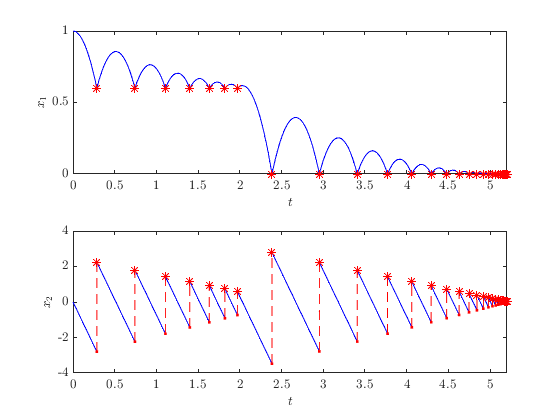
The following plot depicts the hybrid arc for the height of the ball in hybrid time.