Behavior in the Intersection of C and D
This example demonstrates how to define the behavior of simulations in the intersection of the flow and jump sets.
Contents
The files for this example are found in the package hybrid.examples.behavior_in_C_intersection_D :
- initialize.m
- hybrid_priority.slx
- postprocess.m
The contents of this package are located in Examples\+hybrid\+examples\behavior_in_C_intersection_D (clicking this link changes your working directory).
Mathematical Model
Consider the hybrid system with data
\[\begin{array}{ll} f(x) := x & C:= [1, 3] \cup [5, 9] \\ \\ g(x) := \left\{\begin{array}{ll} \mathrm{round}(x+1) & \textrm{if } x \leq 6 \\ 0 & \textrm{if } x = 7 \end{array}\right. & D:= \{0\}\cup [2, 6] \cup \{7\}. \end{array}\]
The sets \(C\) and \(D\) are visualized here:
\[\begin{array}{cccccccccccc} C: & & [ & & ] & & [ & & & & ] \\ D: & * & & [ & & & & ] & * & & \\ \hline x: & 0 & 1 & 2 & 3 & 4 & 5 & 6 & 7 & 8 & 9 \end{array}\]
Solutions to this model are not unique because solutions are allowed to both flow or jump everywhere in \([2, 3) \cup [5, 6] \cup \{7\}.\) (Note that despite \(3\) being in \(C\cap D\) , it is not possible to flow because the trajectory would immediately leave \(C\) .)
Priority Rules for Intersection of C and D
When solving hybrid systems, the HyEQ Toolbox only computes a single solution, so we must specify which of the various possible solutions are computed. This is done is by defining a variable rule in the MATLAB workspace. The value of rule specifies whether flows or jumps have priority in \(C \cap D\) .
- If rule = 1 , jumps have priority.
- If rule = 2 , flows have priority.
- If rule = 3 , then flowing and jumping is randomly selected at each time step.
The following simulations show the use of the variable rule priority of flowing vs jumping when computing solutions inside \(C\cap D\) .
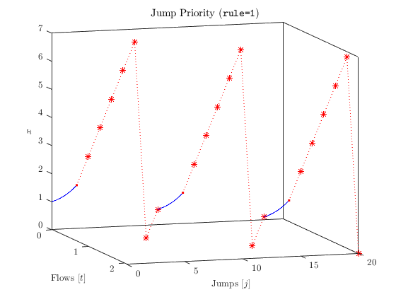
Jump Priority ( rule = 1 )
When rule=1 , jumps have priorty, so anytime a (numerical) solution \(x\) is in \(C\cap D\) , then \(x\) will jump. For the model presented above, this effectively restricts \(C\) as shown here:
\[\begin{array}{rccccccccccc} C \textrm{ (effective)}: & & [ & ) & & & & ( &\circ& & ] \\ D: & * & & [ & & & & ] & * & & \\ \hline x: & 0 & 1 & 2 & 3 & 4 & 5 & 6 & 7 & 8 & 9 \end{array}\]
The following plot shows a solution from \(x0=0\) with jump priority ( rule=1 ). The solution always jumps except when \(x\) is in \([1, 2) \subset C \setminus D\) .

Flow Priority ( rule = 2 )
When rule=2 , flows have priorty, so anytime a solution \(x\) is in \(C\cap D\) , then \(x\) will flow unless \(x\) is on the boundary of \(C\) and \(f(x)\) points out of \(C\) . For the model presented above, this effectively restricts \(C\) as shown here:
\[\begin{array}{rccccccccccc} C: & & [ & & ] & & [ & & & & ] \\ D \textrm{ (effective)}: & * & & & ( & & ) & & & & \\ \hline x: & 0 & 1 & 2 & 3 & 4 & 5 & 6 & 7 & 8 & 9 \end{array}\]
The following plot shows a solution from \(x0=0\) with flow priority ( rule=2 ). The solution only jumps when \(x\) is in \(\{0\} \cup (3, 4) = D \setminus C\) . At the end of the solution, \(x\) leaves \(C \cup D\) and terminates.


Note that the stopping logic is implemented such that when the state of the hybrid system is not in \((C \cup D)\) , then the simulation is stopped. In particular, if this condition becomes true while flowing, then the last value of the computed solution will not belong to \(C\) .
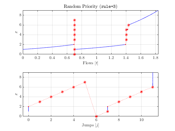
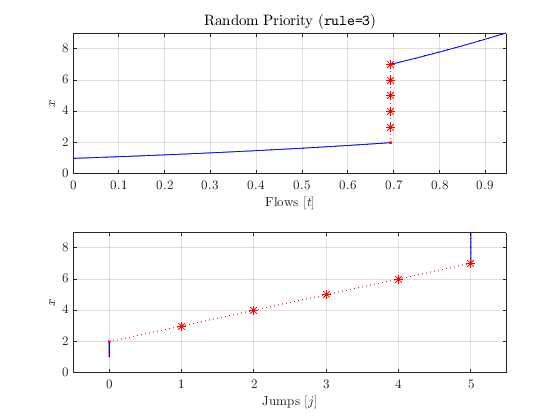
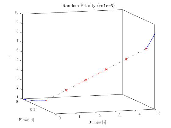
Random Priority ( rule = 3 )
When rule=3 , then at each time step that a solution \(x\) is in \(C \cap D,\) there is 50% chance of jumping and 50% chance of flowing.
For the model presented above, the intersection of \(C\) and \(D\) is illustrated here. Within the intersection, either flowing or jumping can occur in numerical solutions.
\[\begin{array}{cccccccccccc} C \cap D: & & & [ & ] & & [ & ] & * & & \\ \hline x: & 0 & 1 & 2 & 3 & 4 & 5 & 6 & 7 & 8 & 9 \end{array}\]
A solution computed with rule=3 is shown below. The first interval of flow ends around \(t=0.7\) , shortly after the solution enters \([2,3]\) . Because there is a 50-50 chance of jumping at each time step, jumps tend to happen very quickly when a solution enters an interval in \(C \cap D\) . The solution then jumps several times in \(D \setminus C\) until \(x = 7 \in C\cap D\) . The first time this happens, the solution happens to jump, reseting \(x\) to \(0\) , but the second time it happens to flow, causing it to leave \(D\) and eventually leave \(C\) as well.

Numerical Limitations
Isolated points in \(D\) that are also in \(C\) , such as \(x=7\) , require extra care. If a solution starts at x0=6.1 , then it will almost certainly flow pass \(7 \in D\) without jumping (even if rule=1 ) because the odds of the numerical value of x ever being exactly \(7\) is minuscule. Thus, from a numerical standpoint, x never enters \(D\) . Isolated points in \(D\) on the boundary of \(C\) require similar care, as the solution is likely to terminate rather than enter the jump set.
Furthermore, suppose the jump map given above is modified by removing the \(\mathrm{round}\) function, as shown here
\[g(x) := \left\{\begin{array}{ll} x+1 & \textrm{if } x \leq 6 \\ 0 & \textrm{if } x = 7. \end{array}\right. \]
For a solution from x0=1 with jump priority rule=1 , one might expect that a solution will flow until \(x = 2\in D,\) jump several times until \(x=7\in D\) and reset to \(x=0\) . This will not happen, however, because the numerical solver cannot determine the exact position of \(x\) when it enters \(D\) at \(x=2\) , so the solution flows slightly past \(2\) , say, to \(2.0001\) . Then, after several jumps, \(x\) is at \(7.0001 \not\in D\) , at which point it flows until it leaves \(C.\) Therefore, one must be careful in the design of \(C\) and \(D\) to ensure that numerical calculations do not create undesired behavior.