The Integrator System Block
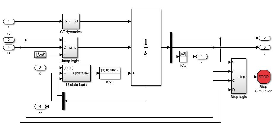
In this page we discuss the internals of the Integrator System block:
Contents
Continuous Time (CT) Dynamics
The block containing the Continuous Time (CT) Dynamics is shown here:
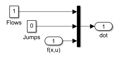
It defines the CT dynamics by assembling the time derivative of the state \([t\ j\ x^\top]^\top\) . States \(t\) and \(j\) are considered states of the system because they need to be updated throughout the simulation in order to keep track of the time and number of jumps. Without \(t\) and \(j\) , solutions could not be plotted accurately. This is given by
\[\left[\begin{array}{c} \dot{t} \\ \dot{j} \\ \dot{x} \end{array}\right] = \left[\begin{array}{c} 1 \\ 0 \\ f(x, u) \end{array}\right]. \]
Note that input port \(1\) takes the value of \(f(x,u)\) through the output of the Embedded MATLAB function block f .
Jump Logic
The inputs to the jump logic block, shown below, are the output of the blocks C and D indicating whether the state is in those sets or not, and a random signal with uniform distribution in \([0,1]\) .
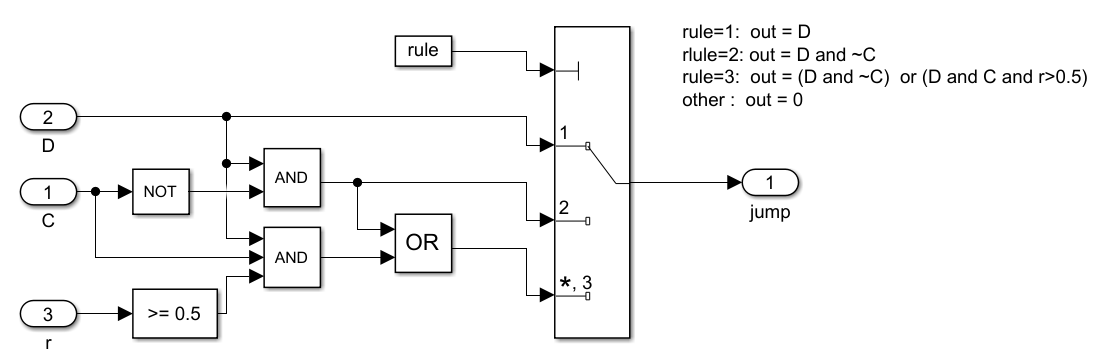
The variable rule defines whether the simulator gives priority to jumps, priority to flows, or no priority. It is initialized in initialize.m .
The output of the Jump Logic is equal to 1 , triggering a jump, when:
- the output of the D block is equal to one and rule=1 ,
- the output of the C block is equal to zero, the output of the D block is equal to one, and rule=2 ,
- the output of the C block is equal to zero, the output of the D block is equal to one, and rule=3 ,
- or the output of the C block is equal to one, the output of the D block is equal to one, rule = 3 , and the random signal \(r\) is larger or equal than \(0.5\) .
Under these events, the output of this block, which is connected to the integrator external reset input, triggers a reset of the integrator, that is, a jump of \(\mathcal{H}\) . The reset or jump is activated since the configuration of the reset input is set to "level hold", which executes resets when this external input is equal to one (if the next input remains set to one, multiple resets would be triggered). Otherwise, the output is equal to zero.
Update Logic
The Update Logic block is shown here:
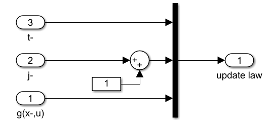
The update logic uses the state port information of the integrator. This port reports the value of the state of the integrator, \([t\ j\ x^\top]^\top\) , at the exact instant that the reset condition becomes true. Notice that \(x^-\) differs from \(x\) since at a jump, \(x^-\) indicates the value of the state that triggers the jump, but it is never assigned as the output of the integrator. In other words, \(x \in D\) is checked using \(x^-\) and if true, \(x\) is reset to \(g(x^-,u)\) . Notice, however, that \(u\) is the same because at a jump, \(u\) indicates the next evaluated value of the input, and it is assigned as the output of the integrator. The flow time \(t\) is kept constant at jumps and \(j\) is incremented by one. More precisely,
\[\left[\begin{array}{c} t^+ \\ j^+ \\ x^+ \end{array}\right] = \left[\begin{array}{c} t^- \\ j^{-}+1 \\ g(x^-,u) \end{array}\right] \]
where \([t^-\ j^-\ {x^-}^\top]^\top\) is the state that triggers the jump.
Stop Logic
The Stop Logic block is shown here:
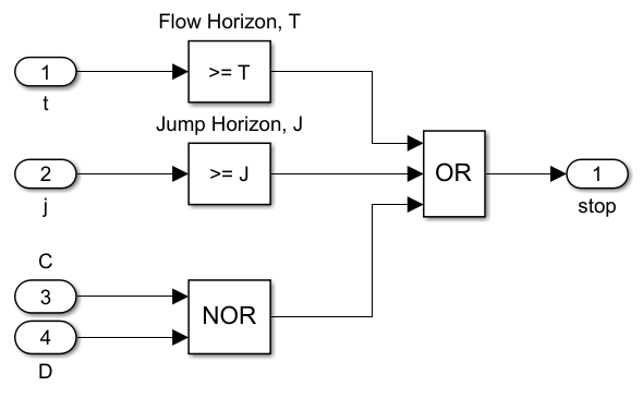
It stops the simulation under any of the following events:
- The flow time is larger than or equal to the maximum flow time specified by \(T\) .
- The jump time is larger than or equal to the maximum number of jumps specified by \(J\) .
- The state of the hybrid system \(x\) is neither in \(C\) nor in \(D\) .
Under any of these events, the output of the logic operator connected to the Stop block becomes one, stopping the simulation. Note that the inputs \(C\) and \(D\) are routed from the output of the blocks computing whether the state is in \(C\) or \(D\) and use the value of \(x^-\) .