Plotting Hybrid Arcs
In this document, we describe how to generate plots of HybridArc objects using HybridPlotBuilder .
Contents
Setup
First, we create several HybridArc solution objects to use as examples
import hybrid.examples.*
config = HybridSolverConfig('Refine', 8); % 'Refine' option makes the plots smoother.
system = BouncingBall();
system_3D = Example3DHybridSystem();
sol = system.solve([10, 0], [0 30], [0 30], config);
sol_3D = system_3D.solve([0; 1; 0], [0, 20], [0, 100], config);
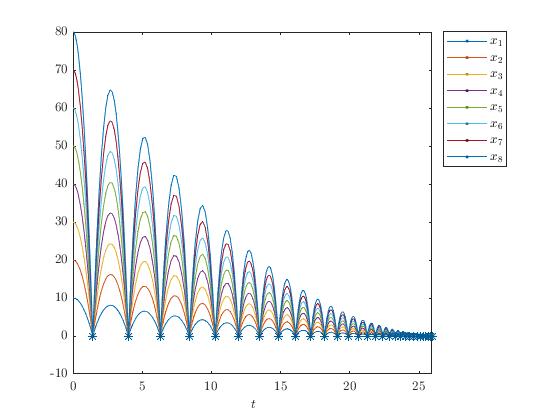
sol_8D = HybridArc(sol.t, sol.j, sol.x(:, 1)*(1:8));
Basic Plotting
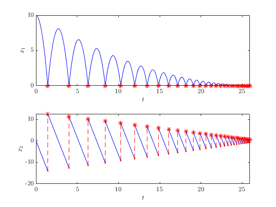
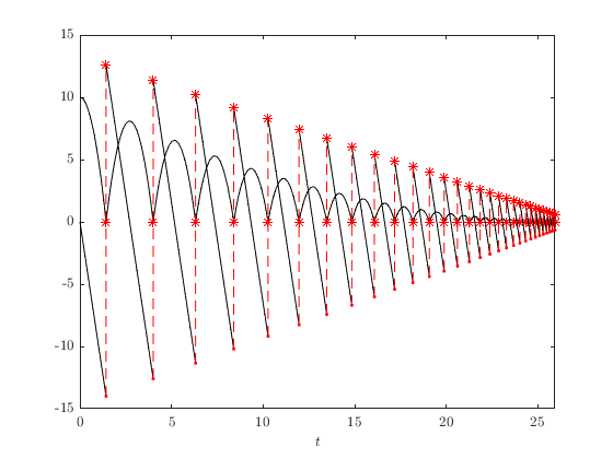
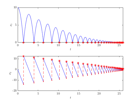
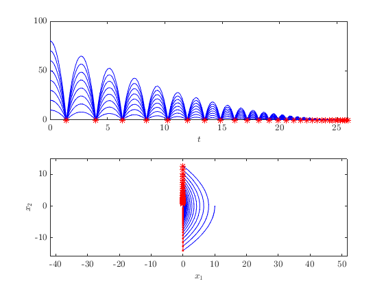
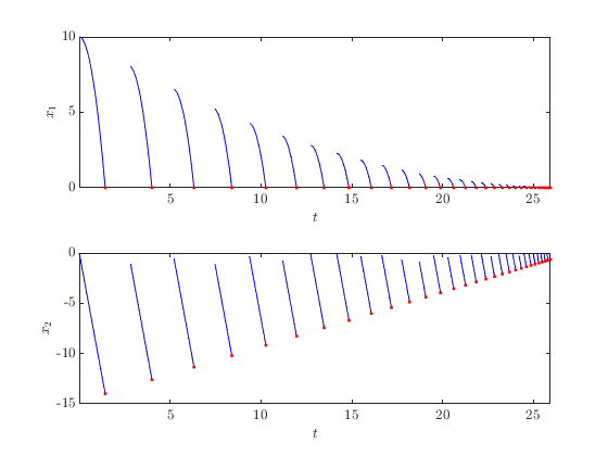
The Hybrid Equations Toolbox provides two approaches to plotting hybrid solutions, depending the level of control required. The first approach, designed for quickly viewing solutions, is to pass a HybridArc object to plotFlows , plotJumps , plotHybrid , or plotPhase . The plotFlows function plots each component of the solution versus discrete time \(t\) .
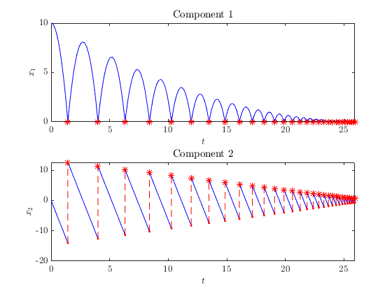
plotFlows(sol); % x vs. t
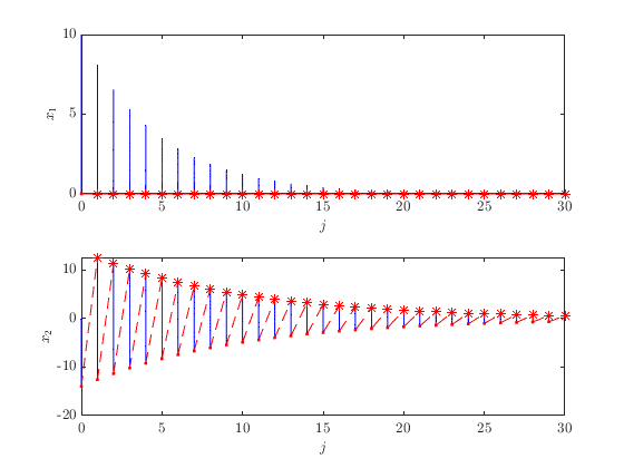
The plotJumps function plots each component of the solution versus discrete time \(j\) .
plotJumps(sol); % x vs. j
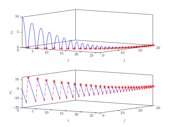
The plotHybrid function plots each component of the solution versus hybrid time \((t, j)\) .
plotHybrid(sol); % x vs. (t, j)
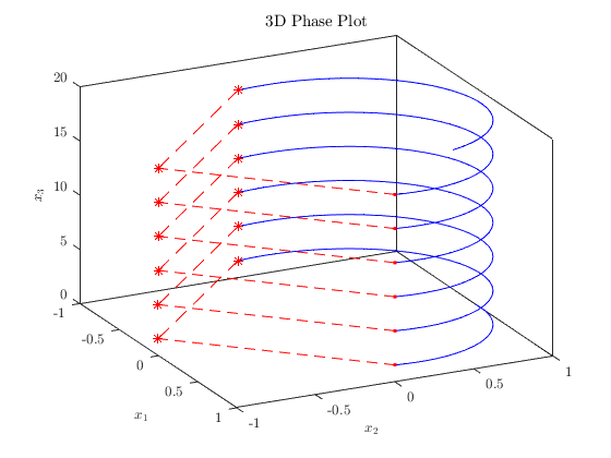
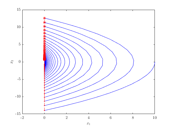
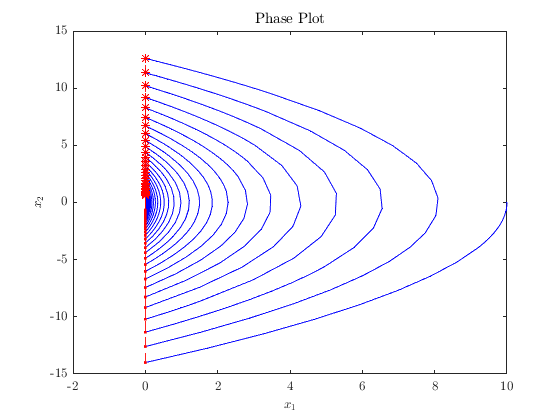
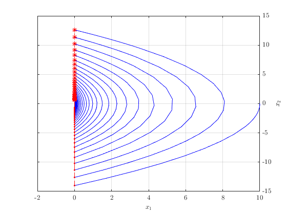
The plotPhase function plots a 2D or 3D solution vector x in phase space.
plotPhase(sol); % x1 vs. x2
title('2D Phase Plot')
snapnow; clf
plotPhase(sol_3D)
title('3D Phase Plot')
view([63.6 28.2]) % Adjust the view angle.

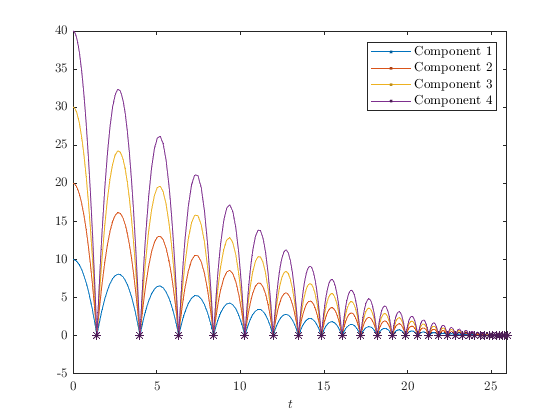
For solutions with four or less components, plotFlows , plotJumps , plotHybrid plot each component in separate subplots, as shown above. Solutions with five or more components are plotted in a single subplot with each colors and a legend included to label each component.
plotFlows(sol_8D)
The second plotting approach is to use the HybridPlotBuilder class explicitly (the first approach also uses HybridPlotBuilder "under the hood" to draw plots). This approach allows for extensive customization and is therefore, better suited for creation of plots for publication. The remainder of this document discusses how to use the second approach. The first step is to create an instance of HybridPlotBuilder .
hpb = HybridPlotBuilder();
Properties are set by calling functions (described below) on the HybridPlotBuilder object.
hpb.flowColor('black'); % Set the flow color to black.
To create a plot, one of the plotting functions plotFlows , plotJumps , plotHybrid , or plotPhase is called. Note that subplots are not created, by default.
hpb.plotFlows(sol)
In MATLAB R2016a and later, if the plot builder is only used once, it can be used immediately without assigning it to a variable by chaining a series of function calls.
HybridPlotBuilder().flowColor('black').plotFlows(sol);
Prior to MATLAB R2016a, function calls cannot be chained directly after a constructor, so the code above must be split into a variable assignment, followed by the function calls:
hpb = HybridPlotBuilder();
hpb.flowColor('black').plotFlows(sol);
Automatic Subplots
Automatic subplots can be enabled by calling HybridPlotBuilder.subplots('on') . When auto-subplots is 'on' and plotFlows , plotJumps , or plotHybrid is called, then a subplot is created for each plotted state component. If, on the otherhand, plotPhase is called, then a single subplot is created. If the current figure did not, previously, have the correct number of subplots, then the figure is cleared before plotting.
HybridPlotBuilder().subplots('on').plotFlows(sol)
When auto-subplots is 'off' , all plots are placed in the current axes (the default value is 'off' ).
clf % clear figure. Otherwise previous subplots are reused.
subplot(2, 1, 1)
HybridPlotBuilder().subplots('off').plotFlows(sol_8D)
subplot(2, 1, 2)
HybridPlotBuilder().subplots('off').plotPhase(sol)
axis padded
axis equal
At this point, if we call a plotting function with auto-subplots 'on' , then the figure is reset to the correct number of subplots.
%    <- No 'clf' here.
HybridPlotBuilder().subplots('on').plotPhase(sol)
Choosing Components to Plot
Often, you may wish to plot only some of the components in a HybridArc object hybrid_arc . To select particular components of hybrid_arc , call hybrid_arc.select(ndxs) where ndxs is a vector containing the indices of the components you wish to plot. Then, simply pass the output to one of the plotting functions. For example, to plot components 1 and 2, pass the array [1, 2] or (equivalently) 1:2 to select .
clf
plotPhase(sol_3D.select([1,2]));
To switch the order of components in the plot, simply switch the order in the array. Note that the labels \(x_1\) and \(x_2\) do not update to reflect the switched order.
HybridPlotBuilder().plotPhase(sol_3D.select([2,1]));
Plotting Other Values
It is possible to plot values contained in an array while using the hybrid time domain from a given HybridArc . To accomplish this, pass a HybridArc object as the first argument to a plotting function and pass the array of values as the second argument. The number of rows in the values array must match the number of entries in sol.t .
clf
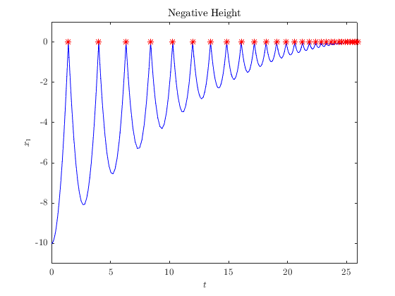
height = sol.x(:, 1); % Extract height component
HybridPlotBuilder().plotFlows(sol, -height) % Plot negative height
title('Negative Height')
ylabel('$x_1$')
ylim padded
Alternatively, a function handle can be evaluated and plotted at each time step in a HybridArc . The evaluation of the function is done via HybridArc.evaluateFunction() .
g = system.gamma; % gravity
HybridPlotBuilder().plotFlows(sol, @(x) g*x(1) + 0.5*x(2)^2);
title('Total Energy')
ylabel('$E$')
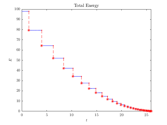
The function handle passed to plotting function must have the input arguments @(x) , @(x, t) or @(x, t, j) and return a column vector.
Customizing Plot Appearance
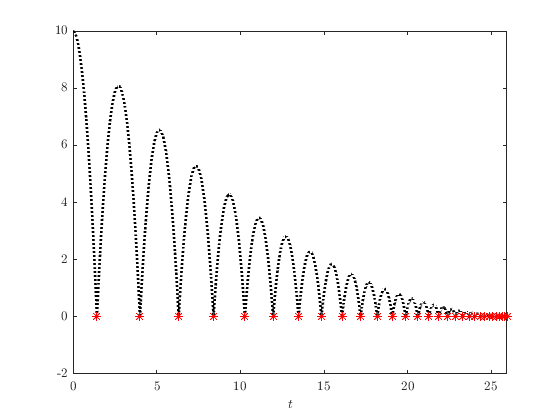
The following functions modify the appearance of flows.
HybridPlotBuilder()...
    .flowColor('black')...
    .flowLineWidth(2)...
    .flowLineStyle(':')...
    .plotFlows(sol.select(1))
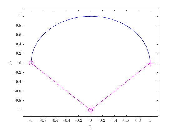
Similarly, we can change the appearance of jumps.
HybridPlotBuilder()...
    .jumpColor('m')... % magenta
    .jumpLineWidth(1)...
    .jumpLineStyle('-.')...
    .jumpStartMarker('+')...
    .jumpStartMarkerSize(16)...
    .jumpEndMarker('o')...
    .jumpEndMarkerSize(10)...
    .plotPhase(sol_3D.select(1:2))
axis padded
To configure the the jump markers on both sides of jumps with a single function call, omit 'Start' and 'End' from the function names:
HybridPlotBuilder()...
    .jumpMarker('s')... % square
    .jumpMarkerSize(12)...
    .plotPhase(sol_3D.select(1:2))
To hide jumps or flows, set the corresponding color to 'none' . To hide jump markers only, but show jump lines set the marker style to 'none' . Similarly, to hide only jump lines, set the jump line style to 'none' .
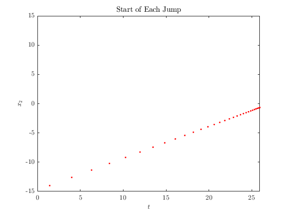
HybridPlotBuilder()...
    .flowColor('none')...
    .jumpEndMarker('none')...
    .jumpLineStyle('none')...
    .plotFlows(sol.select(2))
title('Start of Each Jump') % An alternative way to add titles is shown below.
ylabel('$x_2$')
Sequences of colors can be set by passing a cell array to the color functions. When auto-subplots are off, the color that each component is plotted rotates through the given colors. The following commands create a plot where the first component is plotted with blue flows and red jumps, and the second component is plotted with black flows and green jumps. (If the solution had a third component, the colors would cycle back to blue flows and red jumps.)
clf
HybridPlotBuilder().subplots('off')...
    .flowColor({'blue', 'black'})...
    .jumpColor({'red', 'green'})...
    .legend('Component 1', 'Component 2')... % The 'legend' function is described below.
    .plotFlows(sol);
When auto-subplots are enabled, then all the plots added by a single call to a plotting function are the same color, and all the plots added by the next call to a plotting function are the next color, and so on. Note, here, we set both flow and jump color via the color function. Furthermore, the 'matlab' argument tells HybridPlotBuilder to use the default colors used by MATLAB plots.
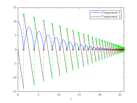
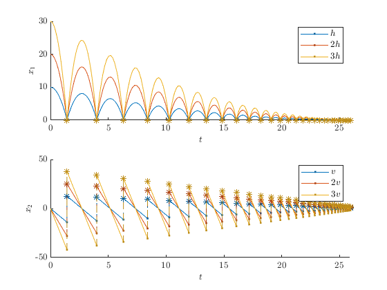
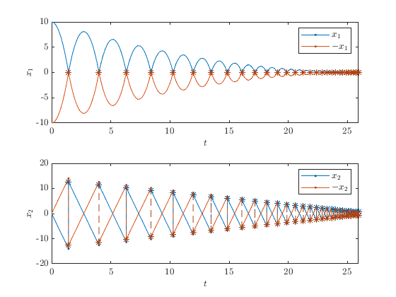
hpb = HybridPlotBuilder().subplots('on').color('matlab');
hold on
hpb.legend('$h$', '$v$').plotFlows(sol);
hpb.legend('$2h$', '$2v$').plotFlows(sol, @(x) 2*x);
hpb.legend('$3h$', '$3v$').plotFlows(sol, @(x) 3*x);
Titles, Labels, and Legends
This section describes how to add text to plots using HybridPlotBuilder . The built-in MATLAB functions for adding labels and titles can also be used, but using HybridPlotBuilder offers the ability to easily configure default settings (text size, interpreter, etc.) and use automatically generated axis labels. The built-in legend function does not work with plots generated by HybridPlotBuilder .
Axis Labels
For state axes, labels are set via the labels function (or, optionally, the label function if there is only one label). Depending on the type of plot and whether auto-subplots is enabled, all components will either be grouped into a single label or each component will have its own label. All components are grouped into a single label if auto-subplots is 'off' and the plot is generated using plotFlows , plotJumps , or plotHybrid (in other words, any plotting function except phasePlot ).
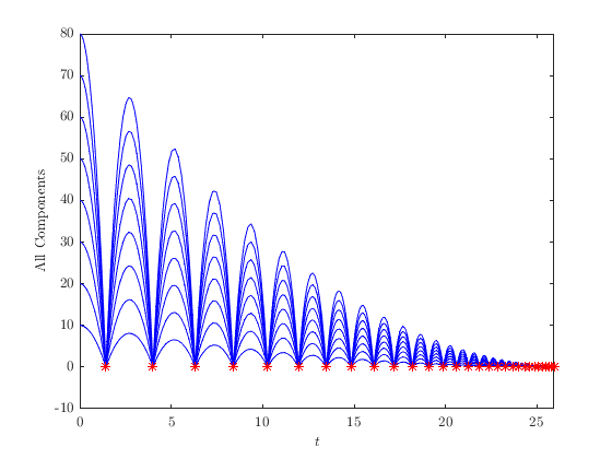
clf
HybridPlotBuilder()...
    .subplots('off')... % This is the default
    .label('All Components')...
    .plotFlows(sol_8D)
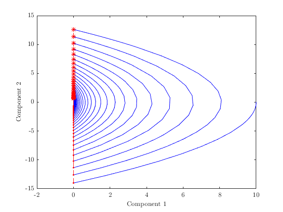
Alternatively, each component has its own label when each component has its own axis —either because each component is placed in its own subplot using auto-subplots or each component has its own axis in a single phase plot produced using plotPhase . In this case, the label for each component is set by passing multiple strings to HybridPlotBuilder.labels() .
clf
HybridPlotBuilder()...
    .labels('Component 1', 'Component 2')...
    .plotPhase(sol)
If there are fewer labels provided than the number of component axes (or no labels are provided at all), then axis labels are automatically generated. The default format is \(x_1\) , \(x_2\) , etc., but this can be modified by passing a format string to the function xLabelFormat . Any occurance of '%d' in the format string is substituted with the index number of the component.
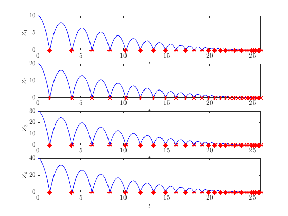
clf
HybridPlotBuilder().subplots('on')...
    .xLabelFormat('$Z_{%d}$')...
    .plotFlows(sol_8D.select(1:4))
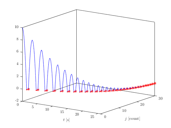
The labels for continuous-time and discrete-time axes (i.e., \(t\) and \(j\) ) can be modified as follows. Using an empty string removes the label.
clf
HybridPlotBuilder()...
    .tLabel('$t$ [s]')...
    .jLabel('$j$ [count]')...
    .plotHybrid(sol.select(1))
Titles
Titles can be set for each subplot via the titles functions (or, optionally, the title function if there is only one title).
clf
HybridPlotBuilder().subplots('on')...
    .titles('Component 1', 'Component 2')...
    .plotFlows(sol)
If auto-subplots is 'off' or a phase plot is generated, then there is only one subplot and thus only one title is used.
clf
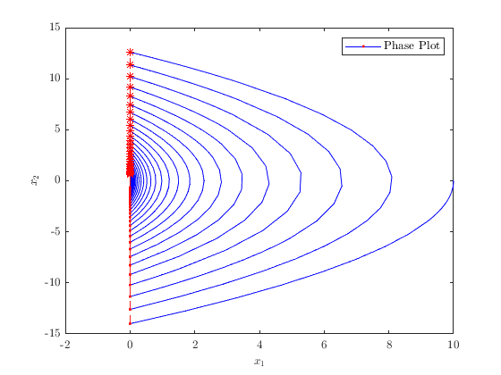
HybridPlotBuilder().title('Phase Plot').plotPhase(sol)
Legend Entries
The function HybridPlotBuilder.legend is used to add legend entries to plots. When using plotPhase , only one legend entry is used.
clf
HybridPlotBuilder().legend('Phase Plot').plotPhase(sol);
Otherwise, when using plotFlows , plotJumps , or plotHybrid , one legend entry is used for each state component (this is true regardless of whether auto-subplots are 'on' or 'off' ).
clf
HybridPlotBuilder().color('matlab')...
    .legend('Component 1', 'Component 2', 'Component 3', 'Component 4')...
    .plotFlows(sol_8D.select(1:4));
Additional plots with legend entries can be added to the same figure by reusing the same HybridPlotBuilder object.
clf
hpb = HybridPlotBuilder().subplots('on').color('matlab');
hpb.legend('$x_1$', '$x_2$').plotFlows(sol);
hold on
hpb.legend('$-x_1$', '$-x_2$').plotFlows(sol.transform(@(x) -x))
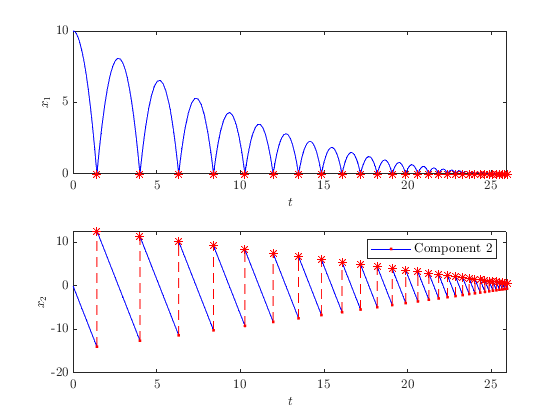
To omit a component from the legend, set the label to an empty string.
clf
HybridPlotBuilder().subplots('on')...
    .legend('', 'Component 2')...
    .plotFlows(sol);
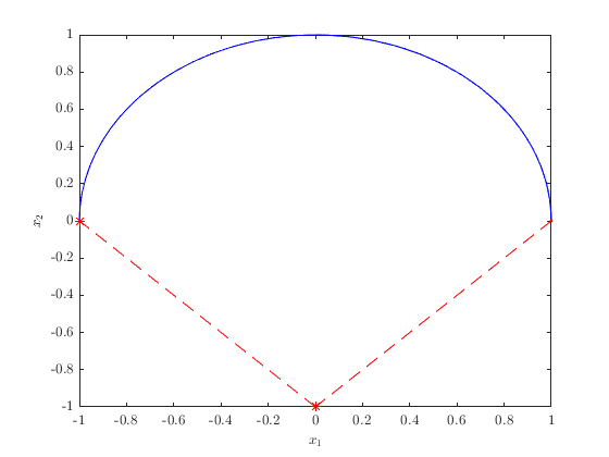
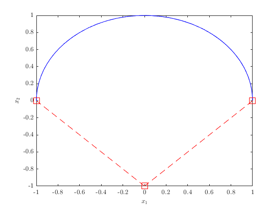
Graphic objects added to a figure without HybridPlotBuilder can be added to the legend by passing the graphic handle to addLegendEntry .
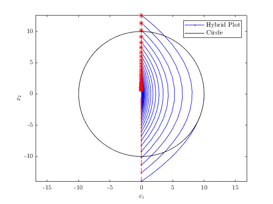
clf
pb = HybridPlotBuilder().legend('Hybrid Plot').plotPhase(sol);
hold on
axis equal

% Plot a circle.
theta = linspace(0, 2*pi);
plt_handle = plot(10*cos(theta), 10*sin(theta), 'black');

% Pass the circle to the plot builder with the desired legend label 'Circle'.
pb.addLegendEntry(plt_handle, 'Circle');
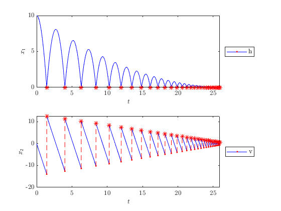
To set legend properties, such as location and number of columns, pass the legend labels to HybridPlotBuilder.legend as a cell array (enclosed with braces '{}') and pass name/value pairs in subsequent arguments. See doc('legend') for a description of legend properties.
clf
HybridPlotBuilder().subplots('on')...
    .legend({'h', 'v'}, 'Location', 'eastoutside')...
    .plotFlows(sol);
Setting the legend options via the methods above applies the same settings to the legends in all subplots. To modify legend options separately for each subplot, use the configurePlots function described below.
Summary of How Many Lables, Titles, and Legend Entries Are Used
In this subsection, we summarize and give examples of how many labels, titles, and legend entries are used, depending on whether auto-subplots are enabled and the choice of plotting function.
| Component Labels | Titles | Legend Entries | |
|---|---|---|---|
Auto-subplots
'off'
|
Single (unless
plotPhase()
)
|
Single | * |
Auto-subplots
'on'
|
Multiple: one label per subplot | Multiple: one title per subplot | * |
plotPhase()
|
Multiple: one label per axis | * | Single |
plotFlows()
,
plotJumps()
, or
plotHybrid()
|
Single (unless auto-subplots is
'on'
)
|
* | Multiple: one legend entry per component |
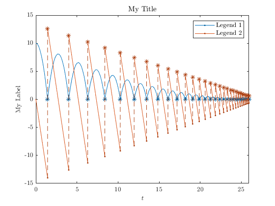
Example: auto-subplots 'off' and using plotFlows , plotJumps or plotHybrid .
clf
HybridPlotBuilder().color('matlab')...
    .subplots('off')... % (default)
    .label('My Label')... % Single: auto-subplots is 'off' and using plotFlows.
    .title('My Title')... % Single: auto-subplots is 'off'.
    .legend('Legend 1', 'Legend 2')... % One per component: using plotFlows
    .plotFlows(sol);
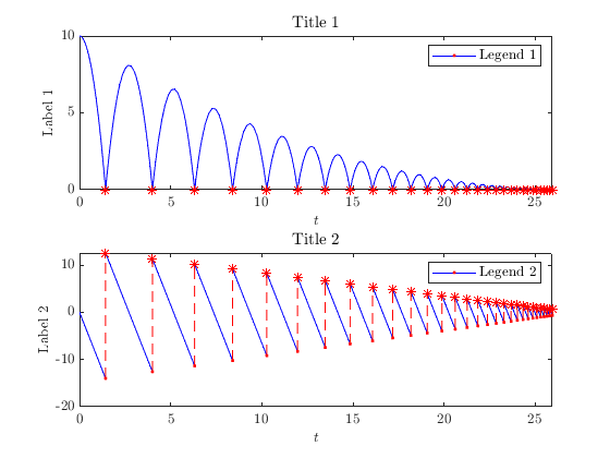
Example: auto-subplots 'on' and using plotFlows , plotJumps or plotHybrid .
clf
HybridPlotBuilder()...
    .subplots('on')...
    .labels('Label 1', 'Label 2')... % One per component: auto-subplots is 'on'
    .titles('Title 1', 'Title 2')... % One per component: auto-subplots is 'on'
    .legend('Legend 1', 'Legend 2')... % One per component: using plotFlows
    .plotFlows(sol);
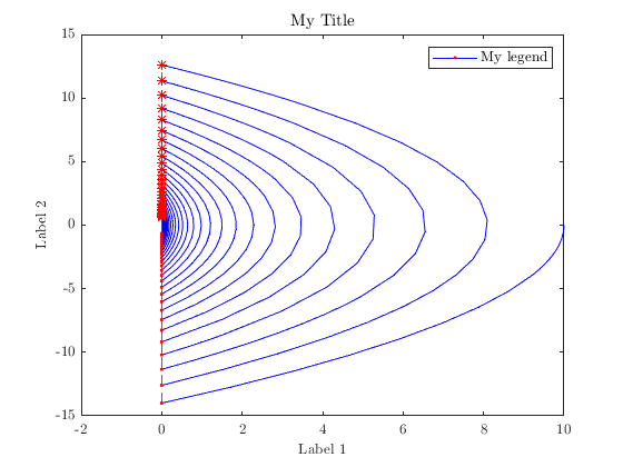
Example: Using plotPhase (auto-subplots has no effect).
clf
HybridPlotBuilder()...
    .labels('Label 1', 'Label 2')... % One per component: using plotPhase
    .title('My Title')... % Single: using plotPhase
    .legend('My legend')... % Single: using plotPhase
    .plotPhase(sol);
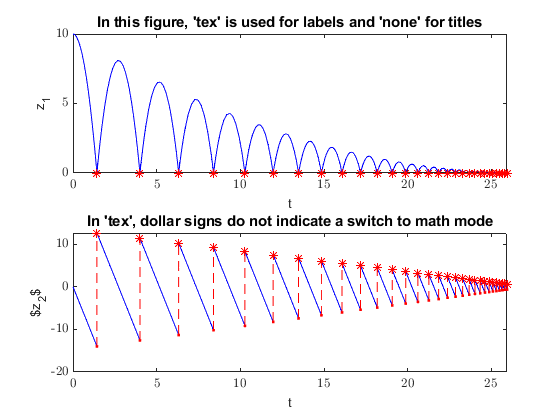
Text Interpreters
The default text interpreter in HybridPlotBuilder is latex . This can be changed by calling HybridPlotBuilder.titleInterpreter() or HybridPlotBuilder.labelInterpreter() with one of these values: 'none' , 'tex' , or 'latex' . The default labels automatically change to match the label interpreter.
HybridPlotBuilder().subplots('on')...
    .titleInterpreter('none')...
    .labelInterpreter('tex')...
    .titles('In this figure, ''tex'' is used for labels and ''none'' for titles',...
            'In ''tex'', dollar signs do not indicate a switch to math mode') ...
    .labels('z_1', '$z_2$')...
    .plotFlows(sol)
Filtering Solutions
Portions of solutions can be hidden with the filter function. In this example, we create a filter that only includes points where the second component (velocity) is negative. (If the time-step size along flows is large, deleted lines connected to filtered points may extends a noticible distance into the portion of the solution that should be visible.)
is_falling = sol.x(:,2) < 0;
HybridPlotBuilder().subplots('on')...
    .filter(is_falling)...
    .plotFlows(sol)
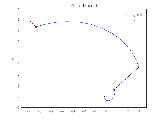
Example: Plotting System Modes
Filtering is useful for plotting systems where an integer-value component indicates the mode of the system. Here, we create a 3D system with a continuous variable \(z \in \mathbb{R}^2\) and a discrete variable \(q \in \{0, 1\}\) . Points in the solution where \(q = 0\) are plotted in blue, and points where \(q = 1\) are plotted in black. The same HybridPlotBuilder object is used for both plots by saving it to the builder variable (this allows us to specify the labels only once and add a legend for both plots).
clf
system_with_modes = hybrid.examples.ExampleModesHybridSystem();


% Create initial condition and solve.
z0 = [-7; 7];
q0 = 0;
sol_modes = system_with_modes.solve([z0; q0], [0, 10], [0, 10], config);

% Extract values for q-component.
q = sol_modes.x(:, 3);

% Plot the [1, 2] components (that is, the first two components) of
% sol_modes at all time steps where q == 0.
builder = HybridPlotBuilder();
builder.title('Phase Portrait') ...
    .labels('$x_1$', '$x_2$') ...
    .legend('$q = 0$') ...
    .filter(q == 0) ... % Only plot points where q is 0.
    .plotPhase(sol_modes.select([1,2]))
hold on % See the section below about 'hold on'
% Plot in black the solution (still only the [1,2] components) for all time
% steps where q == 1.
builder.flowColor('black') ...
    .jumpColor('none') ...
    .legend('$q = 1$') ...
    .filter(q == 1) ... % Only plot points where q is 1.
    .plotPhase(sol_modes.select([1,2]))
axis padded
axis equal
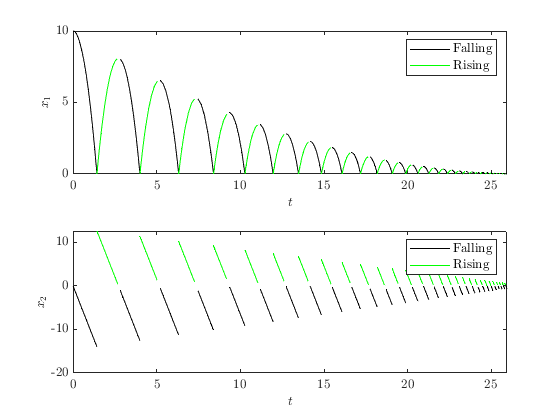
Example: Showing when Bouncing Ball is Rising and Falling
For the bouncing ball system, we can change the color of the plot based on whether the ball is falling.
clf
is_falling = sol.x(:, 2) < 0;
pb = HybridPlotBuilder()....
    .subplots('on')...
    .filter(is_falling)...
    .jumpColor('none')...
    .flowColor('k')...
    .legend('Falling', 'Falling')...
    .plotFlows(sol);
hold on
pb.filter(~is_falling)...
    .flowColor('g')...
    .legend('Rising', 'Rising')...
    .plotFlows(sol);
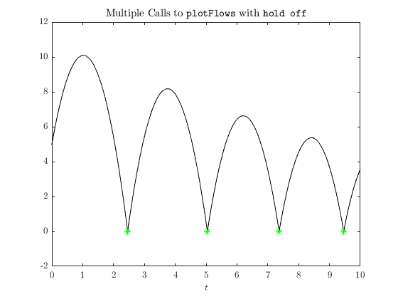
Replacing vs. Adding Plots to a Figure
By default, each call to a HybridPlotBuilder plot function overwrites the previous plots. In the following code, we call plotFlows twice. The first call plots a solution in blue and red, but the second call resets the figure and plots a solution in black and green.
tspan = [0 10];
jspan = [0 30];
sol1 = system.solve([10, 0], tspan, jspan, config);
sol2 = system.solve([ 5, 10], tspan, jspan, config);

clf
HybridPlotBuilder()... % Plots blue flows and red jumps by default.
    .plotFlows(sol1.select(1))
HybridPlotBuilder().flowColor('black').jumpColor('green')...
    .title('Multiple Calls to $\texttt{plotFlows}$ with \texttt{hold off}') ...
    .plotFlows(sol2.select(1))
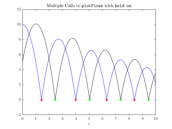
To plot multiple graphs on the same figure, use hold on , similar to standard MATLAB plotting functions.
clf
HybridPlotBuilder().plotFlows(sol1.select(1)) % Plots blue flows and red jumps by default.
hold on
HybridPlotBuilder().flowColor('black').jumpColor('green')...
    .title('Multiple Calls to $\texttt{plotFlows}$ with \texttt{hold on}')...
    .plotFlows(sol2.select(1))
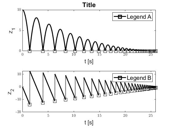
Modifying Defaults
The default values of all HybridPlotBuilder settings can be modified by calling 'set' on the 'defaults' property. The arguments are must be name-value pairs, where the name is a string that matches one of the properties in PlotSettings (names are case insensitive and underscores can be replaced with spaces).
clf
HybridPlotBuilder.defaults.set('auto_subplots', 'on', ...
                             'Label Size', 14, ...
                             'Title Size', 16, ...
                             'label interpreter', 'tex', ...
                             'title interpreter', 'none', ...
                             'flow_color', 'k', ...
                             'flow line width', 2, ...
                             'jump_color', 'k', ...
                             'jump line width', 2, ...
                             'jump line style', ':', ...
                             'jump start marker', 's', ...
                             'jump start marker size', 10, ...
                             'jump end marker', 'none', ...
                             'x_label_format', 'z_{%d}', ...
                             't_label', 't [s]')
HybridPlotBuilder()...
    .title('Title')...
    .legend('Legend A', 'Legend B')...
    .plotFlows(sol);
The defaults can be reset to their original value with the following command.
HybridPlotBuilder.defaults.reset()
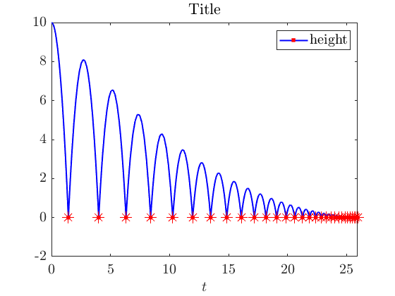
Setting Default Scaling
MATLAB is inconsistent about the size of text and graphics in plots on different devices. To mitigate this difference, three values are included in the settings to adjust the size of text, lines, and markers.
clf
HybridPlotBuilder.defaults.set('text scale', 1.5, ...
                                'line scale', 3, ...
                                'marker scale', 2)
% Example output:
HybridPlotBuilder()...
    .title('Title')...
    .legend('height')...
    .plotFlows(sol.select(1));

HybridPlotBuilder.defaults.reset() % Cleanup
To set the default values in every MATLAB session, create a script named 'startup.m' in the folder returned by the userpath() command. The commands in this script will run every time MATLAB starts.
Additional Configuration
There are numerous options for configuring the appearance of MATLAB plots that are not included explicitly in HybridPlotBuilder (see here ). For plots with a single subplot, the appearance can be modified just like any other MATLAB plot.
HybridPlotBuilder().plotPhase(sol);
grid on
ax = gca;
ax.YAxisLocation = 'right';
Plots with multiple subplots can also be configured as described above by calling subplot(2, 1, 1) and making the desired modifications, then calling subplot(2, 1, 2) , etc., but that approach is messy and tediuous. Instead, the configurePlots function provides a cleaner alternative. A function handle is passed to configurePlots , which is then called by HybridPlotBuilder within each (sub)plot. The function handle passed to configurePlots must take two input arguments. The first is the axes for the subplot and the second is the index for the state component(s) plotted in the plot. For plotFlows , plotJumps , and plotHybrid , this will be one integer, and for phase plots generated with plot , this will be a vector of two or three integers, depending on the dimension of the plot.
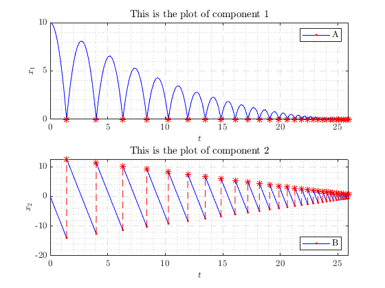
clf
HybridPlotBuilder()...
    .subplots('on')...
    .legend('A', 'B')...
    .configurePlots(@apply_plot_settings)...
    .plotFlows(sol);

function apply_plot_settings(ax, component_ndxs)
    title(ax, sprintf('This is the plot of component %d', component_ndxs))
    % Set the location of the legend in each plot to different positions.
    switch component_ndxs
        case 1
            ax.Legend.Location = 'northeast';
        case 2
            ax.Legend.Location = 'southeast';
    end
    % Configure grid
    grid(ax, 'on')
    grid(ax, 'minor')
    ax.GridLineStyle = '--';
end